
Beam Domain and Delay Domain Sparsity in Wireless Channel Models
In wireless communication, particularly in the context of massive MIMO (Multiple Input Multiple Output) systems and millimeter-wave (mmWave) communication, beam domain and delay domain sparsity are concepts related to the characteristics of the wireless channel.
Beam Domain Sparsity:
In the beam domain, sparsity refers to the phenomenon where only a few beams or beamforming directions experience significant channel gains, while the majority of beams exhibit low channel gains or negligible contributions. This sparsity arises due to the directional nature of beamforming in massive MIMO and mmWave systems. Essentially, beam domain sparsity implies that only a small subset of beams are effective for communication, while the rest can be considered inactive or irrelevant. Exploiting this sparsity allows for efficient beamforming and signal processing algorithms that focus computational resources on the most relevant beams.
Delay Domain Sparsity:
In the delay domain, sparsity refers to the characteristic where the wireless channel exhibits significant energy or power only at certain delay (time) intervals, while the remaining delay intervals have low or negligible channel energy. This sparsity arises due to phenomena such as multipath propagation, where signals arrive at the receiver through multiple paths with different delays. Delay domain sparsity implies that the channel impulse response, which describes how the channel responds to a short-duration input signal, has a sparse representation in the delay domain. Exploiting this sparsity allows for efficient channel estimation and equalization techniques, particularly in scenarios with rich multipath propagation.
In summary, beam domain sparsity and delay domain sparsity are characteristics of wireless channels that arise due to the directional nature of beamforming and the multipath propagation phenomenon, respectively. Exploiting these sparsity properties is essential for designing efficient signal processing algorithms in advanced wireless communication systems.
The tutorial covers the following:
The tutorial will demonstate the following features which are expected characteristics of wireless channels:
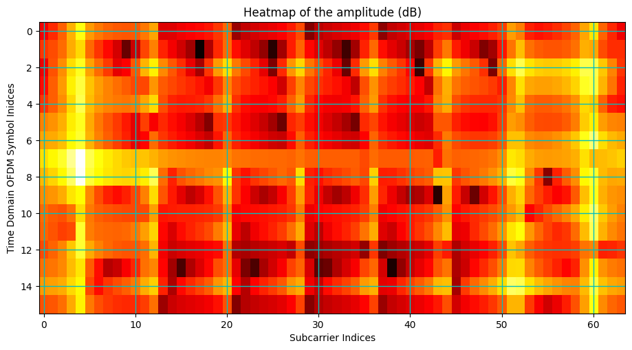
Heatmap of beam domain channel
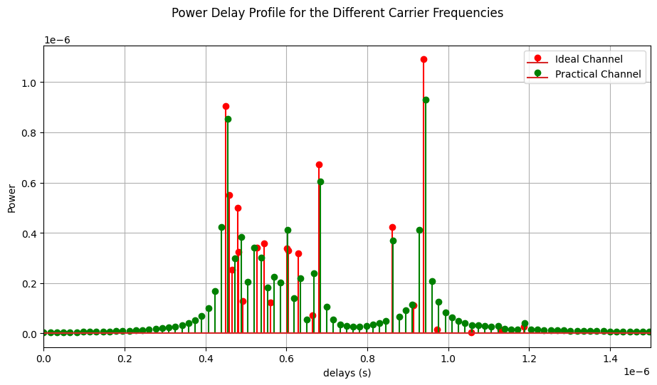
Power delay profile to demonstate the delay domain sparsity
Import Libraries
Import Python Libraries
[1]:
import os
os.environ["CUDA_VISIBLE_DEVICES"] = "-1"
os.environ['TF_CPP_MIN_LOG_LEVEL'] = '3'

# %matplotlib widget
import matplotlib.pyplot as plt
import matplotlib.patches as patches
import matplotlib.animation as animation
import numpy as np
Import 5G Toolkit
[2]:
# importing necessary modules for simulating channel model
import sys
sys.path.append("../../../")
from toolkit5G.ChannelModels import NodeMobility
from toolkit5G.ChannelModels import AntennaArrays
from toolkit5G.ChannelModels import SimulationLayout
[3]:
# from IPython.display import display, HTML
# display(HTML("<style>.container { width:60% !important; }</style>"))
Simulation Parameters
Define the following Simulation Parameters:
propTerraindefines propagation terrain for BS-UE linkscarrierFrequencydefines carrier frequency in HznBSsdefines number of Base Stations (BSs)nUEsdefines number of User Equipments (UEs)nSnapShotsdefines number of SnapShots, where SnapShots correspond to different time-instants at which a mobile user channel is being generated.
[4]:
# Simulation Parameters
propTerrain      = "UMa"         # Propagation Scenario or Terrain for BS-UE links
carrierFrequency = 3.6*10**9     # carrier frequency in Hz
nBSs             = 21            # number of BSs
nUEs             = 10            # number of UEs
Antenna Arrays
Antenna Array at Rx
The following steps describe the procedure to generate AntennaArrays Objects at a single carrier frequency both at Tx and Rx side:
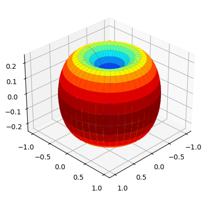
Choose an omni directional dipole antenna for Rx, for which we have to pass the string “OMNI” while instantiating
AntennaArraysclass.Pass
arrayStructureof[1,1,2,2,1]meaning 1 panel in vertical direction, 1 panel in horizonatal direction, 2 antenna elements per column per panel, 2 columns per panel and 1 correspond to antenna element being single polarized.For this antenna structure, the number of Rx antennas
Nrto be 4.
[5]:
# Antenna Array at UE side
# antenna element type to be "OMNI"
# with single panel and 4 single polarized antenna element per panel.
ueAntArray = AntennaArrays(antennaType = "OMNI",
                           centerFrequency = carrierFrequency,
                           arrayStructure  = np.array([1,1,4,4,1]))

ueAntArray()

# num of Rx antenna elements
nr = ueAntArray.numAntennas
# Radiation Pattern of Rx antenna element
fig, ax = ueAntArray.displayAntennaRadiationPattern()
Antenna Array at Tx
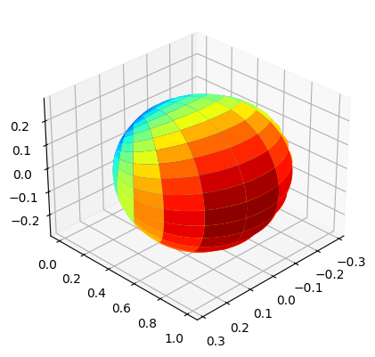
We choose a parabolic antenna for Tx, for which we have to pass the string
"3GPP_38.901"while instantiatingAntennaArraysclass.We pass
arrayStructureof[1,1,2,4,2]meaning 1 panel in vertical direction, 1 panel in horizonatal direction, 2 antenna elements per column per panel, 4 columns per panel and 2 correspond to antenna element being dual polarized.With this structure, we obtain number of Tx antennas
ntto be 16.
[6]:
# Antenna Array at BS side
# antenna element type to be "3GPP_38.901", a parabolic antenna
# with single panel and 8 dual polarized antenna element per panel.


bsAntArray = AntennaArrays(antennaType     = "3GPP_38.901",
                           centerFrequency = carrierFrequency,
                           arrayStructure  = np.array([1,1,8,8,1]))
bsAntArray()

# num of Tx antenna elements
nt = bsAntArray.numAntennas
# Radiation Pattern of Tx antenna element
fig, ax = bsAntArray.displayAntennaRadiationPattern()
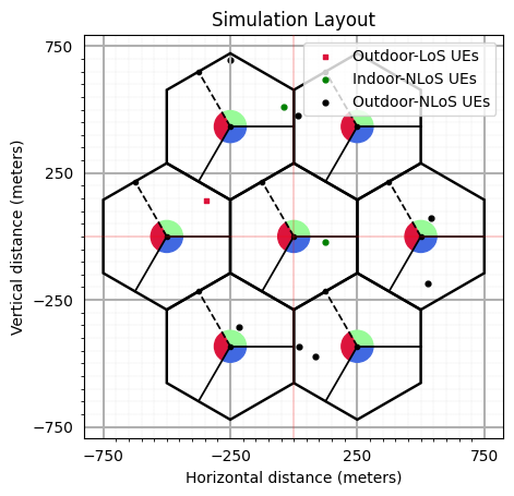
Simulation Layout
We define the simulation topology parametes:
ISD: Inter Site DistanceminDist: Minimum distance between transmitter and receiver.bsHt: BS heightsueHt: UE heightstopology: Simulation TopologynSectorsPerSite: Number of Sectors Per Site
Furthermore, users can access and update following parameters as per their requirements for channel using the handle simLayoutObj.x where x is:
The following parameters can be accessed or updated immendiately after object creation
UEtracksUELocationsueOrientationUEvelocityVectorBStracksBSLocationsbsOrientationBSvelocityVector
The following parameters can be accessed or updated after calling the object
linkStateVec
[7]:
# Layout Parameters
isd             = 500         # inter site distance
minDist         = 35          # min distance between each UE and BS
ueHt            = 1.5         # UE height
bsHt            = 35          # BS height
topology        = "Hexagonal" # BS layout type
nSectorsPerSite = 3           # number of sectors per site


# simulation layout object
simLayoutObj = SimulationLayout(numOfBS = nBSs,
                                numOfUE = nUEs,
                                heightOfBS = bsHt,
                                heightOfUE = ueHt,
                                ISD = isd,
                                layoutType = topology,
                                numOfSectorsPerSite = nSectorsPerSite)

# Update UE location for motion over a circle centered around the BS location.
# simLayoutObj.UELocations = -simLayoutObj.UEtracks.mean(0)

simLayoutObj(terrain = propTerrain,
             carrierFreq = carrierFrequency,
             ueAntennaArray = ueAntArray,
             bsAntennaArray = bsAntArray,
             forceLOS = False)

# displaying the topology of simulation layout

fig, ax = simLayoutObj.display2DTopology()
      enableSpatialConsistency: True
               memoryEfficient: False
enableSpatialConsistencyIndoor: True
Channel Parameters, Channel Coefficients and OFDM Channel
The user can access the channel coefficents and other parameters using following handles:
LSPs/SSPs: paramGenObj.x where x is
linkStateVecdelaySpreadphiAoA_LoS,phiAoA_mn,phiAoA_spreadthetaAoA_LoS,thetaAoA_mn,thetaAoA_spreadphiAoD_LoS,phiAoD_mn,phiAoD_spreadthetaAoD_LoS,thetaAoD_mn,thetaAoD_spreadxprpathloss,pathDelay,pathPowershadowFading
Channel Co-efficeints: channel.x where x is
coefficientsdelays
Shape of OFDM Channel:
Hfis of shape :(number of carrier frequencies, number of snapshots, number of BSs, number of UEs, Nfft, number of Rx antennas, number of Tx antennas)
[8]:
# Generate SSPs/LSPs Parameters:
paramGenObj = simLayoutObj.getParameterGenerator()

# Generate Channel Coefficeints and Delays: SSPs/LSPs
channel = paramGenObj.getChannel(applyPathLoss = True)
# Channel coefficients can be accessed using: channel.coefficients
# Channel delays can be accessed using:       channel.delays

# Generate OFDM Channel
Nfft = 2048
Hf   = channel.ofdm(30*10**3, Nfft, simLayoutObj.carrierFrequency)
[Warning]: Pathloss model for UMa is defined only for BS height 'hBS' = 25! Ignoring for now but might results in unexpected behaviour!
[Warning]: UE height 'hUE' cannot be less than 1.5! These values are forced to 1.5! for 'UMa'
[Warning]: Pathloss model for UMa is defined only for BS height 'hBS' = 25! Ignoring for now but might results in unexpected behaviour!
[Warning]: UE height 'hUE' cannot be less than 1.5! These values are forced to 1.5! for 'UMa'
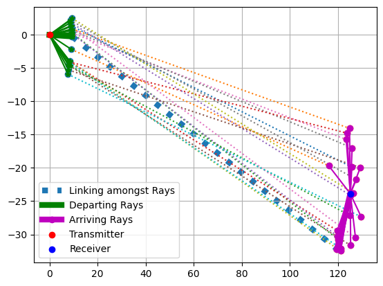
[9]:
fig, ax = paramGenObj.displayClusters(indices=(0, 1, 0), rayIndex=1, carrierIndex=0,
                                      radiusRx=10, radiusTx=10, displayPlot=False)
[10]:
Hf.shape
[10]:
(1, 1, 21, 10, 2048, 16, 64)
Demonstrating the Beam Domain Sparsity
[11]:
bsIndex = 0
ueIndex = 0
scIndex = 0
Nt      = Hf.shape[-1]
Nr      = Hf.shape[-2]
overSamplingFactorTx = 4
overSamplingFactorRx = 4

Ftx = np.fft.ifft(np.eye(overSamplingFactorTx*Nt), overSamplingFactorTx*Nt)[0:Nt]
Frx = np.fft.ifft(np.eye(overSamplingFactorRx*Nr), overSamplingFactorRx*Nr)[:,0:Nr]

Hbeam = Frx@Hf[0,0,bsIndex,ueIndex,scIndex]@Ftx
Hbeam = np.fft.fft(np.fft.fft(Hf[0,0,bsIndex,ueIndex,scIndex], axis = -1), axis = -2)
[12]:
fig, ax = plt.subplots(figsize = (11,5.5))

carrierIndex = 0
bsIndex      = 0
ueIndex      = 0
bsAntIndex   = 0
ueAntIndex   = 0

ax.imshow(10*np.log10(np.abs(Hbeam)), cmap = 'hot', interpolation='nearest', aspect = "auto")
ax = plt.gca();
ax.grid(color='c', linestyle='-', linewidth=1)
ax.set_xlabel("Subcarrier Indices")
ax.set_ylabel("Time Domain OFDM Symbol Inidces")
ax.set_title("Heatmap of the amplitude (dB)")

# Gridlines based on minor ticks
plt.show()
Demonstrating the Delay Domain Sparsity
[16]:
bsIndex   = 0
ueIndex   = 0
txAntenna = 0
rxAntenna = 0

Nt      = Hf.shape[-1]
Nr      = Hf.shape[-2]
overSamplingFactorTx = 4
overSamplingFactorRx = 4

ht       = np.fft.ifft(Hf[0,0,bsIndex,ueIndex,:,rxAntenna,txAntenna], n = Nfft, axis=0, norm = "ortho")
[18]:
fig, ax = plt.subplots(figsize = (11,5.5))

carrierIndex = 0
snapIndex    = 0
bsIndex      = 0
ueIndex      = 0
bsAntIndex   = 0
ueAntIndex   = 0

tau = channel.delays[0,0,bsIndex,ueIndex]

ax.stem(tau, np.abs(channel.coefficients[0,0,bsIndex,ueIndex,:,ueAntIndex,bsAntIndex]), "r", label = "Ideal Channel")
ax.stem(np.arange(Nfft)/(Nfft*channel.subCarrierSpacing), np.abs(ht), "g", label = "Practical Channel")
ax.legend()
ax.set_xlim([0, 0.15*10**-5])
ax.set_xlabel("delays (s)")
ax.set_ylabel("Power")
ax.grid()

fig.suptitle("Power Delay Profile for the Different Carrier Frequencies")
plt.show()
[ ]: