Constellation Learning in an AWGN Channel

In this notebook, we will learn how to implement an end-to-end digital communication system as an AutoEncoder[1] and compared its performance with a (n,k) Hamming Code.

We analyze the performance of an autoencoder based modeling of a communication system as opposed to traditional modeling, where designing signal alphabet at transmitter (Tx) and detection algorithms at receiver (Rx) are based on a given mathematical/statistical channel/system model.
We simulate the performance of an AutoEncoder based communication link in the presence of Additive White Gaussian Noise (AWGN), where Tx sends one out of M message/information symbols per n channel uses through a noisy channel and the Rx estimates the transmitted symbols through noisy observations.
The goal is to learn a signalling alphabet/constellation scheme that is robust with respect to the noise introduced by the channel at Tx

## Table of Contents

Importing Libraries
Parameters of AE
Training Data
Testing Data
Normalization Functions
Defining AE Model
Training AE
Defining Tx, Channel and Rx from Trained AE
Constellation Learning
Block Error Rate (BLER) performance
References

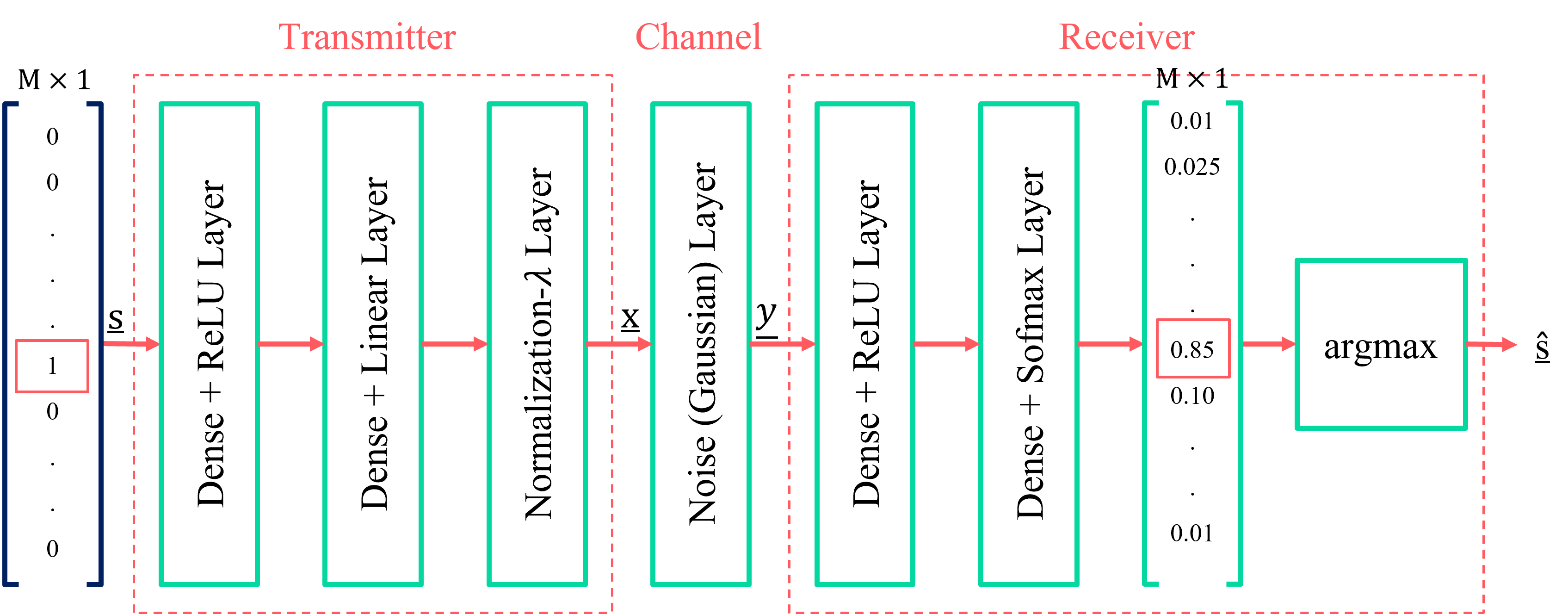
PHY layer as AutoEncoder

The fundamental idea behind this tutorial is to model Physical Layer as an AutoEncoder(AE).
An AutoEncoder(AE) is an Artificial Neural Network (ANN) used to learn an efficient representation of data at an intermediate layer to reproduce the input at its output.
We Interpret end to end communication link, i.e., Tx, channel, and Rx as a single Neural Network (NN) that can be trained as an AE which reconstructs its input at its output, as communication is all about reproducing/reconstructing messages transmitted by Tx at Rx faithfully in the presence of channel perturbations and Rx noise.

Steps

Following are the steps that we follow in simulation:

Define the hyper parameters of AE :
- number of information symbols M, where each symbol carry kbits
- number of channel uses n
- snr in dB at which AE is being trained, which we call snr_train
Define embedings for each information symbol that is to be fed as an input to AE.
Define training and testing data set by randomizing the label
Define end to end AutoEncoder by using the already imported keras built in layers.
- Tx is being implmented as a stack of two keras Dense layers one with ReLU activation and another with linear activation. The output of the second Dense layer is fed to a normalization layer which we implement using keras Lambda layer.
- Channel is implemented as a single Noise layer with certain noise standard deviation, which is a function of both Rate of the code (R) and snr_train.
- Rx also consists of two keras Dense layers, one with ReLU activation and the last one with softmax activation. The last layer must output probabilities (i.e., for a given received noisy vector v of dimension M, it outputs max aposteriori probability vector of dimension M, i.e., max(prob(w|v)) for any w belongs to transmitted oneshot embeddings)

Note: We choose different values of number of training (N) and testing samples (N_test) for constellation plots and for BlockErrorRate (BLER) plots.

Note: For (n,k) = (7,4), we use sklearn T-distributed Stochastic Neighbor Embedding (TSNE) to plot the learned constellation. Typically we use less number of N and N_test in such cases. For BLER plots we always go with high values of N, N_test

Importing Libraries

[1]:

import os
os.environ["CUDA_VISIBLE_DEVICES"] = "-1"
os.environ['TF_CPP_MIN_LOG_LEVEL'] = '3'


# Importing necessary Numpy, Matplotlib, TensorFlow, Keras and scikit-learn modules
# %matplotlib widget
# %matplotlib inline
import matplotlib.pyplot as plt
import numpy as np
import tensorflow as tf
from keras.layers import Input, Dense, GaussianNoise, Lambda, BatchNormalization
from keras.models import Model
from keras.optimizers import Adam, SGD
from keras import backend as be

[2]:

import sys
sys.path.append(".")
from toolkit5G.SymbolMapping import Demapper
from toolkit5G.SymbolMapping import Mapper
from toolkit5G.ChannelCoder  import HammingEncoder
from toolkit5G.ChannelCoder  import HammingDecoder

The following code cell defines the parametes of an AutoEncoder including the snr_dB at which it is being trained. We assume (n,k) = (7,4) here but the code is generailized to support other configurations as well such as (2,4) and (2,2) given in [1]

Parameters of AutoEncoder

[3]:

#################################################
# Parameters of a (n,k) AutoEncoder (AE)
# all the symbols are assumed to be real valued
#################################################

# number of information/message symbols that Tx communicates over channel to Rx
M = 16
# number of bits per information symbol
k = int(np.log2(M))
# number of channel uses or dimension of each code-word symbol or number of bits per code-word symbol
n = 7
# Rate of communication. i.e., k bits per n channel uses
R = k/n
print("###################################################################################################")
print("Parameters of "+str((n,k))+" AutoEncoder are:\n")
print("Number of Information Symbols:" + str(M))
print("Number of Bits Per Information Symbol:" + str(k))
print("Number of Channel Uses:" + str(n))
print("Rate of Communication:" + str(R))

###################################################################################################
Parameters of (7, 4) AutoEncoder are:

Number of Information Symbols:16
Number of Bits Per Information Symbol:4
Number of Channel Uses:7
Rate of Communication:0.5714285714285714

[4]:

###################################
#SNR at which AE is being trained
###################################
#---------------------------------------------------------------------------------------------------------------
# SNR in dB = Es/No, where Es: Energy per symbol, No: Noise Power Spectral Density
snr_dB = 7
# snr in linear scale
snr_train = np.power(10,snr_dB/10)
# noise standard deviation
noise_stddev = np.sqrt(1/(2*R*snr_train))

Training Data

[5]:

#############################################
# One-hot embeddings of information symbols.
#############################################
# Each information symbol is mapped to a standard basis vector of dimension M

symbol_encodings = np.eye(M)
print("One-Hot Encodings of information symbols:\n")
print(symbol_encodings)

One-Hot Encodings of information symbols:

[[1. 0. 0. 0. 0. 0. 0. 0. 0. 0. 0. 0. 0. 0. 0. 0.]
 [0. 1. 0. 0. 0. 0. 0. 0. 0. 0. 0. 0. 0. 0. 0. 0.]
 [0. 0. 1. 0. 0. 0. 0. 0. 0. 0. 0. 0. 0. 0. 0. 0.]
 [0. 0. 0. 1. 0. 0. 0. 0. 0. 0. 0. 0. 0. 0. 0. 0.]
 [0. 0. 0. 0. 1. 0. 0. 0. 0. 0. 0. 0. 0. 0. 0. 0.]
 [0. 0. 0. 0. 0. 1. 0. 0. 0. 0. 0. 0. 0. 0. 0. 0.]
 [0. 0. 0. 0. 0. 0. 1. 0. 0. 0. 0. 0. 0. 0. 0. 0.]
 [0. 0. 0. 0. 0. 0. 0. 1. 0. 0. 0. 0. 0. 0. 0. 0.]
 [0. 0. 0. 0. 0. 0. 0. 0. 1. 0. 0. 0. 0. 0. 0. 0.]
 [0. 0. 0. 0. 0. 0. 0. 0. 0. 1. 0. 0. 0. 0. 0. 0.]
 [0. 0. 0. 0. 0. 0. 0. 0. 0. 0. 1. 0. 0. 0. 0. 0.]
 [0. 0. 0. 0. 0. 0. 0. 0. 0. 0. 0. 1. 0. 0. 0. 0.]
 [0. 0. 0. 0. 0. 0. 0. 0. 0. 0. 0. 0. 1. 0. 0. 0.]
 [0. 0. 0. 0. 0. 0. 0. 0. 0. 0. 0. 0. 0. 1. 0. 0.]
 [0. 0. 0. 0. 0. 0. 0. 0. 0. 0. 0. 0. 0. 0. 1. 0.]
 [0. 0. 0. 0. 0. 0. 0. 0. 0. 0. 0. 0. 0. 0. 0. 1.]]

[6]:

###############################################################################
# Generating data samples of size N. Each sample can take values from 0 to M-1
###############################################################################
N  = 9600000
#*********************************************************************************
# use this value of N only for Constellation plot when using TSNE under (7,4) AE
# N = 1500
#*********************************************************************************
# random indices for labeling information symbols
train_label = np.random.randint(M,size=N)
print(train_label)

[ 1  8  4 ... 10  1 10]

[7]:

########################
# Training data samples
########################
data = []
for i in train_label:
    temp = np.zeros(M)
    temp[i] = 1
    data.append(temp)
# converting data in to a numpy array
train_data = np.array(data)
print("\n")
# Printing the shape of training data
print("The shape of training data:")
print(train_data.shape)



The shape of training data:
(9600000, 16)

[8]:

# Verifying training data with its label or index for 13 samples

tempLabel_train = np.random.randint(N,size=13)
print(tempLabel_train)
print("\n")
for i in tempLabel_train:
    print(train_label[i],train_data[i])

[6634013 5698954 7797983 1647048 8484082 5849713 6844526 1561517 3625133
 6378228 3180495 1370770 5104703]


11 [0. 0. 0. 0. 0. 0. 0. 0. 0. 0. 0. 1. 0. 0. 0. 0.]
7 [0. 0. 0. 0. 0. 0. 0. 1. 0. 0. 0. 0. 0. 0. 0. 0.]
15 [0. 0. 0. 0. 0. 0. 0. 0. 0. 0. 0. 0. 0. 0. 0. 1.]
14 [0. 0. 0. 0. 0. 0. 0. 0. 0. 0. 0. 0. 0. 0. 1. 0.]
15 [0. 0. 0. 0. 0. 0. 0. 0. 0. 0. 0. 0. 0. 0. 0. 1.]
10 [0. 0. 0. 0. 0. 0. 0. 0. 0. 0. 1. 0. 0. 0. 0. 0.]
12 [0. 0. 0. 0. 0. 0. 0. 0. 0. 0. 0. 0. 1. 0. 0. 0.]
8 [0. 0. 0. 0. 0. 0. 0. 0. 1. 0. 0. 0. 0. 0. 0. 0.]
13 [0. 0. 0. 0. 0. 0. 0. 0. 0. 0. 0. 0. 0. 1. 0. 0.]
11 [0. 0. 0. 0. 0. 0. 0. 0. 0. 0. 0. 1. 0. 0. 0. 0.]
9 [0. 0. 0. 0. 0. 0. 0. 0. 0. 1. 0. 0. 0. 0. 0. 0.]
2 [0. 0. 1. 0. 0. 0. 0. 0. 0. 0. 0. 0. 0. 0. 0. 0.]
3 [0. 0. 0. 1. 0. 0. 0. 0. 0. 0. 0. 0. 0. 0. 0. 0.]

Testing Data

[9]:

###############################
# Generating data for testing
###############################
N_test = 16000
#**************************************************
# use this only for Constellation Plot of (7,4) AE
# N_test = 500
#**************************************************
test_label = np.random.randint(M,size=N_test)
test_data = []
for i in test_label:
    temp    = np.zeros(M)
    temp[i] = 1
    test_data.append(temp)
# converting it to a numpy array
test_data = np.array(test_data)
# Printing the shape of test data
print("The shape of test data is:")
print(test_data.shape)

The shape of test data is:
(16000, 16)

[10]:

# Verifying test data with its label for 7 sample
tempTestLabel = np.random.randint(N_test,size=7)
print(tempTestLabel)
print("\n")
for i in tempTestLabel:
    print(test_label[i],test_data[i])

[11519  4498 10702  6711  2993  9873  5688]


4 [0. 0. 0. 0. 1. 0. 0. 0. 0. 0. 0. 0. 0. 0. 0. 0.]
2 [0. 0. 1. 0. 0. 0. 0. 0. 0. 0. 0. 0. 0. 0. 0. 0.]
3 [0. 0. 0. 1. 0. 0. 0. 0. 0. 0. 0. 0. 0. 0. 0. 0.]
13 [0. 0. 0. 0. 0. 0. 0. 0. 0. 0. 0. 0. 0. 1. 0. 0.]
9 [0. 0. 0. 0. 0. 0. 0. 0. 0. 1. 0. 0. 0. 0. 0. 0.]
3 [0. 0. 0. 1. 0. 0. 0. 0. 0. 0. 0. 0. 0. 0. 0. 0.]
6 [0. 0. 0. 0. 0. 0. 1. 0. 0. 0. 0. 0. 0. 0. 0. 0.]

Normalization Functions

[11]:

def normalizeAvgPower(x):
    """ Normalizes the power of input tensor"""
    return x/(be.sqrt(be.mean(x**2)))

[12]:

def normalizeEnergy(x):
    """ Normalizes the energy of input tensor"""
    return np.sqrt(n)*(be.l2_normalize(x,axis=-1))

Defining AutoEncoder Model

[13]:

##########################################
# Defining AutoEncoder and its layers
##########################################
#----------------------------------------------------------------------------------------------------------------
###########
# Tx layer
###########
onehot  = Input(shape=(M,))
dense1  = Dense(M, activation = 'relu')(onehot)
dense2  = Dense(n, activation = 'linear')(dense1)
x       = Lambda(normalizeAvgPower)(dense2)      # Avg power constraint
# x       = Lambda(normalizeEnergy)(dense2)      # Energy constraint
#****************************************************************************************
################
# Channel Layer
################
y       = GaussianNoise(stddev = noise_stddev)(x)
#****************************************************************************************
###########
# Rx layer
###########
dense3  = Dense(M, activation = 'relu')(y)
prob    = Dense(M, activation = 'softmax')(dense3)
#-----------------------------------------------------------------------------------------------------------------
#########################################
# Defining end to end AutoEncoder Model
#########################################
autoEncoder = Model(onehot, prob)
#-----------------------------------------------------------------------------------------------------------------
# Instantiate optimizer
adam        = Adam(learning_rate=0.01)
# Instantiate Stochastic Gradient Descent Method
sgd         = SGD(learning_rate=0.02)
#-----------------------------------------------------------------------------------------------------------------
# compile end to end model
autoEncoder.compile(optimizer=adam, loss='categorical_crossentropy')
#-----------------------------------------------------------------------------------------------------------------
# printing summary of layers and its trainable parameters
print(autoEncoder.summary())

Model: "model"
_________________________________________________________________
 Layer (type)                Output Shape              Param #
=================================================================
 input_1 (InputLayer)        [(None, 16)]              0

 dense (Dense)               (None, 16)                272

 dense_1 (Dense)             (None, 7)                 119

 lambda (Lambda)             (None, 7)                 0

 gaussian_noise (GaussianNo  (None, 7)                 0
 ise)

 dense_2 (Dense)             (None, 16)                128

 dense_3 (Dense)             (None, 16)                272

=================================================================
Total params: 791 (3.09 KB)
Trainable params: 791 (3.09 KB)
Non-trainable params: 0 (0.00 Byte)
_________________________________________________________________
None

In the following code snippet we show how to train an end to end AE by a call to fit() method specifying the training and validation data. We choose 50 epochs with a batch_size of 1024. One can vary these values to obtain a different trainable model.

Training AutoEncoder

[14]:

#######################
# Training Auto Encoder
########################
autoEncoder.fit(train_data, train_data,
                epochs = 50,
                batch_size = 8*1024,
                validation_data=(test_data, test_data))

Epoch 1/50
1172/1172 [==============================] - 5s 3ms/step - loss: 0.0619 - val_loss: 1.8036e-06
Epoch 2/50
1172/1172 [==============================] - 4s 3ms/step - loss: 0.0016 - val_loss: 1.1638e-07
Epoch 3/50
1172/1172 [==============================] - 4s 3ms/step - loss: 0.0011 - val_loss: 7.2494e-09
Epoch 4/50
1172/1172 [==============================] - 3s 3ms/step - loss: 9.0464e-04 - val_loss: 0.0000e+00
Epoch 5/50
1172/1172 [==============================] - 4s 3ms/step - loss: 7.9008e-04 - val_loss: 0.0000e+00
Epoch 6/50
1172/1172 [==============================] - 3s 3ms/step - loss: 7.7934e-04 - val_loss: 0.0000e+00
Epoch 7/50
1172/1172 [==============================] - 3s 3ms/step - loss: 7.0910e-04 - val_loss: 0.0000e+00
Epoch 8/50
1172/1172 [==============================] - 3s 3ms/step - loss: 6.8701e-04 - val_loss: 0.0000e+00
Epoch 9/50
1172/1172 [==============================] - 3s 3ms/step - loss: 6.5150e-04 - val_loss: 0.0000e+00
Epoch 10/50
1172/1172 [==============================] - 3s 3ms/step - loss: 6.3850e-04 - val_loss: 0.0000e+00
Epoch 11/50
1172/1172 [==============================] - 3s 3ms/step - loss: 6.4894e-04 - val_loss: 0.0000e+00
Epoch 12/50
1172/1172 [==============================] - 3s 3ms/step - loss: 5.9537e-04 - val_loss: 0.0000e+00
Epoch 13/50
1172/1172 [==============================] - 3s 3ms/step - loss: 5.8190e-04 - val_loss: 0.0000e+00
Epoch 14/50
1172/1172 [==============================] - 3s 3ms/step - loss: 5.9939e-04 - val_loss: 0.0000e+00
Epoch 15/50
1172/1172 [==============================] - 3s 3ms/step - loss: 5.6062e-04 - val_loss: 0.0000e+00
Epoch 16/50
1172/1172 [==============================] - 3s 3ms/step - loss: 5.6521e-04 - val_loss: 0.0000e+00
Epoch 17/50
1172/1172 [==============================] - 3s 3ms/step - loss: 5.4805e-04 - val_loss: 0.0000e+00
Epoch 18/50
1172/1172 [==============================] - 3s 3ms/step - loss: 5.6737e-04 - val_loss: 0.0000e+00
Epoch 19/50
1172/1172 [==============================] - 3s 3ms/step - loss: 5.5437e-04 - val_loss: 0.0000e+00
Epoch 20/50
1172/1172 [==============================] - 3s 3ms/step - loss: 5.3964e-04 - val_loss: 0.0000e+00
Epoch 21/50
1172/1172 [==============================] - 3s 3ms/step - loss: 5.1038e-04 - val_loss: 0.0000e+00
Epoch 22/50
1172/1172 [==============================] - 3s 3ms/step - loss: 5.5104e-04 - val_loss: 0.0000e+00
Epoch 23/50
1172/1172 [==============================] - 3s 3ms/step - loss: 5.2465e-04 - val_loss: 0.0000e+00
Epoch 24/50
1172/1172 [==============================] - 3s 3ms/step - loss: 5.3718e-04 - val_loss: 0.0000e+00
Epoch 25/50
1172/1172 [==============================] - 3s 3ms/step - loss: 5.2150e-04 - val_loss: 0.0000e+00
Epoch 26/50
1172/1172 [==============================] - 3s 3ms/step - loss: 5.2325e-04 - val_loss: 0.0000e+00
Epoch 27/50
1172/1172 [==============================] - 3s 3ms/step - loss: 5.2213e-04 - val_loss: 0.0000e+00
Epoch 28/50
1172/1172 [==============================] - 3s 3ms/step - loss: 5.0728e-04 - val_loss: 0.0000e+00
Epoch 29/50
1172/1172 [==============================] - 3s 3ms/step - loss: 5.0278e-04 - val_loss: 0.0000e+00
Epoch 30/50
1172/1172 [==============================] - 3s 3ms/step - loss: 5.3612e-04 - val_loss: 0.0000e+00
Epoch 31/50
1172/1172 [==============================] - 3s 3ms/step - loss: 5.0515e-04 - val_loss: 0.0000e+00
Epoch 32/50
1172/1172 [==============================] - 3s 3ms/step - loss: 5.1903e-04 - val_loss: 0.0000e+00
Epoch 33/50
1172/1172 [==============================] - 3s 3ms/step - loss: 5.2265e-04 - val_loss: 0.0000e+00
Epoch 34/50
1172/1172 [==============================] - 3s 3ms/step - loss: 4.9100e-04 - val_loss: 0.0000e+00
Epoch 35/50
1172/1172 [==============================] - 3s 3ms/step - loss: 4.7689e-04 - val_loss: 0.0000e+00
Epoch 36/50
1172/1172 [==============================] - 3s 3ms/step - loss: 4.8344e-04 - val_loss: 0.0000e+00
Epoch 37/50
1172/1172 [==============================] - 3s 3ms/step - loss: 4.7145e-04 - val_loss: 0.0000e+00
Epoch 38/50
1172/1172 [==============================] - 3s 3ms/step - loss: 4.9232e-04 - val_loss: 0.0000e+00
Epoch 39/50
1172/1172 [==============================] - 3s 3ms/step - loss: 4.5073e-04 - val_loss: 0.0000e+00
Epoch 40/50
1172/1172 [==============================] - 3s 3ms/step - loss: 4.7231e-04 - val_loss: 0.0000e+00
Epoch 41/50
1172/1172 [==============================] - 3s 3ms/step - loss: 4.4049e-04 - val_loss: 0.0000e+00
Epoch 42/50
1172/1172 [==============================] - 3s 3ms/step - loss: 4.3347e-04 - val_loss: 0.0000e+00
Epoch 43/50
1172/1172 [==============================] - 3s 3ms/step - loss: 4.5009e-04 - val_loss: 0.0000e+00
Epoch 44/50
1172/1172 [==============================] - 3s 3ms/step - loss: 4.5302e-04 - val_loss: 0.0000e+00
Epoch 45/50
1172/1172 [==============================] - 3s 3ms/step - loss: 4.3693e-04 - val_loss: 0.0000e+00
Epoch 46/50
1172/1172 [==============================] - 3s 3ms/step - loss: 4.4082e-04 - val_loss: 0.0000e+00
Epoch 47/50
1172/1172 [==============================] - 3s 3ms/step - loss: 4.4123e-04 - val_loss: 0.0000e+00
Epoch 48/50
1172/1172 [==============================] - 3s 3ms/step - loss: 4.5702e-04 - val_loss: 0.0000e+00
Epoch 49/50
1172/1172 [==============================] - 3s 3ms/step - loss: 4.3058e-04 - val_loss: 0.0000e+00
Epoch 50/50
1172/1172 [==============================] - 3s 3ms/step - loss: 4.3849e-04 - val_loss: 0.0000e+00

[14]:

<keras.src.callbacks.History at 0x29775d74b80>

Defining Tx, Channel and Rx from Trained AutoEncoder

[15]:

########################################################
# Defining Tx from end to end trained autoEncoder model
#######################################################

transmitter   = Model(onehot, x)
#*********************************************************
#######################
# Defining channel part
#######################
channelInput  = Input(shape=(n,))
channelOutput = autoEncoder.layers[-3](channelInput)
channel       = Model(channelInput, channelOutput)
#*********************************************************
##################
# Defining Rx part
##################
rxInput       = Input(shape=(n,))
rx1           = autoEncoder.layers[-2](rxInput)
rxOutput      = autoEncoder.layers[-1](rx1)
receiver      = Model(rxInput,rxOutput)

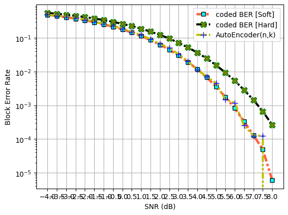
Block Error Rate (BLER) performance

The following code snippet computes and plots BLER performance of of (n,k) AE and compares it with base line (n,k) Hamming code.

Note: Run the following code snippets only with high values of N, N_test. Comment all the following code snippet for constellation plots. Uncomment only for BLER plots

[16]:

#######################################
# SNR vs BLER computation and plotting
#######################################
# use this snr_dB = np.arange(0,15,2) for (n,k) = (2,4) or (2,2) AE
# use this snr_dB = np.arange(-4,8.5,0.5) for (7,4) AE

snr_dB = np.arange(-4,8.5,0.5)
bler   = np.zeros(snr_dB.shape[0])
for ii in range(0,snr_dB.shape[0]):
    snr_linear      = 10.0**(snr_dB[ii]/10.0)      # snr in linear scale
    noise_std       = np.sqrt(1/(2*R*snr_linear))
    noise_mean      = 0
    num_errors      = 0
    num_samples     = N_test
    #-------------------------------------------------------------
    noise           = noise_std*np.random.randn(num_samples,n)
    #-------------------------------------------------------------
    #########################
    # predicted input symbols
    #########################
    x_hat           = transmitter.predict(test_data)
    #-------------------------------------------------------------
    ##############
    # noisy input
    ##############
    x_hat_noisy     = x_hat + noise
    #-------------------------------------------------------------
    ##########################
    # predicted output symbols
    ##########################
    y_hat           = receiver.predict(x_hat_noisy)
    #-------------------------------------------------------------
    ##################
    # symbol estimates
    ##################
    sym_estimates   = np.argmax(y_hat, axis=1)
    #-------------------------------------------------------------
    #################################################
    # counting errors and computing bler at each snr
    #################################################
    num_errors      = int(np.sum(sym_estimates != test_label))
    bler[ii]        = num_errors/num_samples
    print('SNR(dB):', snr_dB[ii], 'BLER:', bler[ii])

500/500 [==============================] - 0s 517us/step
500/500 [==============================] - 0s 503us/step
SNR(dB): -4.0 BLER: 0.498375
500/500 [==============================] - 0s 564us/step
500/500 [==============================] - 0s 567us/step
SNR(dB): -3.5 BLER: 0.458625
500/500 [==============================] - 0s 587us/step
500/500 [==============================] - 0s 522us/step
SNR(dB): -3.0 BLER: 0.4203125
500/500 [==============================] - 0s 567us/step
500/500 [==============================] - 0s 555us/step
SNR(dB): -2.5 BLER: 0.38725
500/500 [==============================] - 0s 515us/step
500/500 [==============================] - 0s 566us/step
SNR(dB): -2.0 BLER: 0.3485625
500/500 [==============================] - 0s 543us/step
500/500 [==============================] - 0s 556us/step
SNR(dB): -1.5 BLER: 0.3043125
500/500 [==============================] - 0s 557us/step
500/500 [==============================] - 0s 662us/step
SNR(dB): -1.0 BLER: 0.2595
500/500 [==============================] - 0s 529us/step
500/500 [==============================] - 0s 535us/step
SNR(dB): -0.5 BLER: 0.2265625
500/500 [==============================] - 0s 556us/step
500/500 [==============================] - 1s 1ms/step
SNR(dB): 0.0 BLER: 0.1879375
500/500 [==============================] - 0s 515us/step
500/500 [==============================] - 0s 540us/step
SNR(dB): 0.5 BLER: 0.152
500/500 [==============================] - 0s 536us/step
500/500 [==============================] - 0s 518us/step
SNR(dB): 1.0 BLER: 0.122375
500/500 [==============================] - 0s 548us/step
500/500 [==============================] - 0s 529us/step
SNR(dB): 1.5 BLER: 0.092
500/500 [==============================] - 0s 560us/step
500/500 [==============================] - 0s 551us/step
SNR(dB): 2.0 BLER: 0.0673125
500/500 [==============================] - 0s 578us/step
500/500 [==============================] - 0s 544us/step
SNR(dB): 2.5 BLER: 0.0513125
500/500 [==============================] - 0s 555us/step
500/500 [==============================] - 0s 512us/step
SNR(dB): 3.0 BLER: 0.03275
500/500 [==============================] - 0s 568us/step
500/500 [==============================] - 0s 553us/step
SNR(dB): 3.5 BLER: 0.02025
500/500 [==============================] - 0s 523us/step
500/500 [==============================] - 0s 538us/step
SNR(dB): 4.0 BLER: 0.011375
500/500 [==============================] - 0s 520us/step
500/500 [==============================] - 0s 515us/step
SNR(dB): 4.5 BLER: 0.0071875
500/500 [==============================] - 0s 504us/step
500/500 [==============================] - 0s 549us/step
SNR(dB): 5.0 BLER: 0.0045625
500/500 [==============================] - 0s 567us/step
500/500 [==============================] - 0s 528us/step
SNR(dB): 5.5 BLER: 0.0015
500/500 [==============================] - 0s 533us/step
500/500 [==============================] - 0s 539us/step
SNR(dB): 6.0 BLER: 0.0011875
500/500 [==============================] - 0s 575us/step
500/500 [==============================] - 0s 536us/step
SNR(dB): 6.5 BLER: 0.00025
500/500 [==============================] - 0s 555us/step
500/500 [==============================] - 0s 522us/step
SNR(dB): 7.0 BLER: 0.000125
500/500 [==============================] - 0s 489us/step
500/500 [==============================] - 0s 527us/step
SNR(dB): 7.5 BLER: 0.000125
500/500 [==============================] - 0s 536us/step
500/500 [==============================] - 0s 510us/step
SNR(dB): 8.0 BLER: 0.0

Hamming Codes

Transmitter

[17]:

##############################
## Hamming Code Configurations
##############################
## (n,k) code for any random positive integer m
m = 3
k = 2**m - m - 1
n = 2**m - 1
#------------------------------------------------
## Payload Generation
numDim = 2
n1     = 1000000
bits   = np.random.randint(2, size = (n1,k))

#-------------------------------------------------
## Hamming Encoder
encBits = HammingEncoder(k,n)(bits)

## Rate Matching
codeword = encBits

## Symbol Mapping
constellation_type  = "bpsk"
num_bits_per_symbol = 1

mapperObject        = Mapper(constellation_type, num_bits_per_symbol)
symbols             = mapperObject(codeword)

print()
print("******** ("+str(n)+","+str(k)+") Hamming Code ********")
print("       Shape of Input:"+str(bits.shape))
print("    Shape of Enc Bits:"+str(encBits.shape))
print("   Constellation type: "+str(constellation_type))
print("Number of bits/symbol: "+str(num_bits_per_symbol))
print("*********************************")
print()


******** (7,4) Hamming Code ********
       Shape of Input:(1000000, 4)
    Shape of Enc Bits:(1000000, 7)
   Constellation type: bpsk
Number of bits/symbol: 1
*********************************

[18]:

######################################
# (7,4) Hamming code BLER performance
######################################

SNR  = 10**(snr_dB/10)  # SNR in linear scale

codedBLERhard = np.zeros(SNR.shape)
codedBLERsoft = np.zeros(SNR.shape)

## Symbol Demapping
# demapping_method = str(np.random.choice(["app", "maxlog"]))
# hard_out         = bool(np.random.choice([False, True]))
demapping_method = "app"
hard_out         = False

demapper         = Demapper(demapping_method, constellation_type,
                            num_bits_per_symbol, hard_out = hard_out)


snrIndex = 0
for snr in SNR:
    symbs = symbols + np.sqrt(0.5/R/snr)*(np.random.standard_normal(size=symbols.shape)+1j*np.random.standard_normal(size=symbols.shape)).astype(np.complex64)

    llrEst  = demapper([symbs, np.float32(1/snr)])
    uncBits = np.where(llrEst > 0, np.int8(1), np.int8(0))

    decoder = HammingDecoder(k,n)
    decBits = decoder(uncBits)

    codedBLERhard[snrIndex]= np.mean(np.where(np.sum(np.abs(bits-decBits), axis=1)>0, True, False))

    decoder = HammingDecoder(k,n)
    decBits = decoder(llrEst, "sphereDecoding")

    codedBLERsoft[snrIndex]= np.mean(np.where(np.sum(np.abs(bits-decBits), axis=1)>0, True, False))

    print("At SNR(dB): "+str(snr_dB[snrIndex])+" | coded BLER (soft): "+str(codedBLERsoft[snrIndex])+" | coded BLER(hard): "+str(codedBLERhard[snrIndex]))

    snrIndex += 1

At SNR(dB): -4.0 | coded BLER (soft): 0.487595 | coded BLER(hard): 0.554942
At SNR(dB): -3.5 | coded BLER (soft): 0.450965 | coded BLER(hard): 0.522681
At SNR(dB): -3.0 | coded BLER (soft): 0.413592 | coded BLER(hard): 0.49012
At SNR(dB): -2.5 | coded BLER (soft): 0.373975 | coded BLER(hard): 0.454293
At SNR(dB): -2.0 | coded BLER (soft): 0.334565 | coded BLER(hard): 0.416966
At SNR(dB): -1.5 | coded BLER (soft): 0.29465 | coded BLER(hard): 0.378652
At SNR(dB): -1.0 | coded BLER (soft): 0.254375 | coded BLER(hard): 0.340119
At SNR(dB): -0.5 | coded BLER (soft): 0.215441 | coded BLER(hard): 0.301021
At SNR(dB): 0.0 | coded BLER (soft): 0.17943 | coded BLER(hard): 0.261749
At SNR(dB): 0.5 | coded BLER (soft): 0.145708 | coded BLER(hard): 0.225524
At SNR(dB): 1.0 | coded BLER (soft): 0.114448 | coded BLER(hard): 0.189009
At SNR(dB): 1.5 | coded BLER (soft): 0.086905 | coded BLER(hard): 0.154485
At SNR(dB): 2.0 | coded BLER (soft): 0.063574 | coded BLER(hard): 0.123722
At SNR(dB): 2.5 | coded BLER (soft): 0.045241 | coded BLER(hard): 0.095985
At SNR(dB): 3.0 | coded BLER (soft): 0.030357 | coded BLER(hard): 0.072166
At SNR(dB): 3.5 | coded BLER (soft): 0.019361 | coded BLER(hard): 0.052022
At SNR(dB): 4.0 | coded BLER (soft): 0.011799 | coded BLER(hard): 0.036823
At SNR(dB): 4.5 | coded BLER (soft): 0.006764 | coded BLER(hard): 0.024702
At SNR(dB): 5.0 | coded BLER (soft): 0.003584 | coded BLER(hard): 0.015639
At SNR(dB): 5.5 | coded BLER (soft): 0.001758 | coded BLER(hard): 0.009331
At SNR(dB): 6.0 | coded BLER (soft): 0.000827 | coded BLER(hard): 0.005393
At SNR(dB): 6.5 | coded BLER (soft): 0.000329 | coded BLER(hard): 0.00284
At SNR(dB): 7.0 | coded BLER (soft): 0.000129 | coded BLER(hard): 0.001444
At SNR(dB): 7.5 | coded BLER (soft): 4.9e-05 | coded BLER(hard): 0.000658
At SNR(dB): 8.0 | coded BLER (soft): 6e-06 | coded BLER(hard): 0.000263

BLER plot : comparison of AutoEncoder BLER with base line (n,k) Hamming Code BLER

[19]:

# ploting BLER
fig, ax = plt.subplots()

ax.semilogy(snr_dB, codedBLERsoft, 'tomato', lw = 3.5, linestyle = (0, (3, 1, 1, 1, 1, 1)), marker = "s", ms = 6, mec = "k", mfc = "cyan", label = "coded BER [Soft]")
ax.semilogy(snr_dB, codedBLERhard, 'k', lw = 3, linestyle = (0, (3, 1, 1, 1, 1, 1)), marker = "X", ms = 9, mec = "green", mfc = "olive", label = "coded BER [Hard]")
ax.semilogy(snr_dB, bler, 'y', lw = 3, linestyle = (0, (3, 1, 1, 1, 1, 1)), marker = "+", ms = 9, mec = "blue", mfc = "pink", label = "AutoEncoder(n,k)")
ax.legend()
ax.set_xticks(snr_dB)
ax.grid()
ax.set_ylabel("Block Error Rate")
ax.set_xlabel("SNR (dB)")

plt.show()

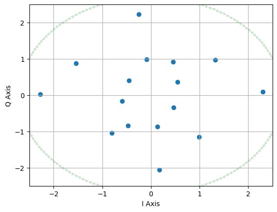
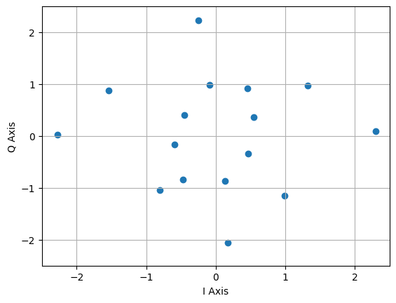
../../../_images/api_Projects_Project7_E2E_Learning_for_Physical_Layer_39_0.png

Constellation Learning

The following cells provide the code to generate and plot the learned constellation by Tx in the presence of AWGN.

Note: we have to go back to the previous steps to change the values of N,N_test and retrain the AE to plot a constellation for (7,4) AE as it uses TSNE. For other cases such as (2,4) and (2,2) we can use same N,N_test for BLER and constellation plots.

[20]:

# #################################################################################
# # predicting the learned constellation for a given number of information symbols M
# #################################################################################
# constellationPoints = transmitter.predict(symbol_encodings)
# print("\n")
# print(constellationPoints)
# print("\n")
# print("Shape of learned constellation:" + str(constellationPoints.shape))

learned constellation plot

[21]:

###################################################################################
# plotting learned constellation under energy constraint for (n,k) = (2,4) or (2,2)
###################################################################################
constellationPoints = transmitter.predict(symbol_encodings)
r = np.linalg.norm(constellationPoints[0])
theta = np.linspace(0,2*np.pi,200)
fig, ax = plt.subplots()
ax.scatter(constellationPoints[:,0],constellationPoints[:,1])
ax.plot(r*np.cos(theta),r*np.sin(theta), c="green", alpha = 0.1, marker=".")
plt.axis((-2.5,2.5,-2.5,2.5))
plt.grid()
plt.xlabel('I Axis')
plt.ylabel('Q Axis')
plt.show()

1/1 [==============================] - 0s 31ms/step

../../../_images/api_Projects_Project7_E2E_Learning_for_Physical_Layer_44_1.png

[22]:

##########################################################################################
# plotting learned constellation under average power constraint for (n,k) = (2,4) or (2,2)
##########################################################################################

fig, ax = plt.subplots()
ax.scatter(constellationPoints[:,0],constellationPoints[:,1])
plt.axis((-2.5,2.5,-2.5,2.5))
plt.grid()
plt.xlabel('I Axis')
plt.ylabel('Q Axis')
plt.show()

../../../_images/api_Projects_Project7_E2E_Learning_for_Physical_Layer_45_0.png

The following code snippet use TSNE to reduce the dimension of constellation for (n,k) = (7,4)

[23]:

# ###########################################################################################################
# # Using sklearn T-distributed Stochastic Neighbor Embedding (TSNE) to reduce the dimension of constellation
# ###########################################################################################################
# num_samples = N_test

# noise       = noise_stddev*np.random.randn(num_samples,n)
# X           = transmitter.predict(test_data)
# X_noisy     = X + noise

# X_embedded  = TSNE(n_components=2, learning_rate='auto', n_iter = 35000, random_state = 0, perplexity=60).fit_transform(X_noisy)
# X_embedded  = X_embedded/n

[24]:

# ####################################################################################
# # plotting higher dimensional received constellation in lower dimensions for (7,4) AE
# ####################################################################################
# fig, ax = plt.subplots()
# ax.scatter(X_embedded[:,0],X_embedded[:,1], marker = ".")
# plt.axis((-2,2,-2,2))
# plt.grid()
# plt.xlabel('I Axis')
# plt.ylabel('Q Axis')
# plt.show()

It turns out that under M = 16 and with an energy constraint, (2,4) AE learns a constellation which resemble 16-ary PSK and with power constraint it learns a constellation which resemble 16-ary APSK.

References

[1] T. O’Shea and J. Hoydis, “An Introduction to Deep Learning for the Physical Layer,” in IEEE Transactions on Cognitive Communications and Networking, vol. 3, no. 4, pp. 563-575, Dec. 2017, doi: 10.1109/TCCN.2017.2758370.

[ ]: