
Channel Generation for Dual Mobility Scenarios in 5G and Beyond
The 5G networks are designed to support scenrios where both transmitter and receiver are moving. Such scenarios are very common in device to device (D2D) and vehicle to everything (V2X) use-cases. The dual mobility results in dual Doppler primarily because of the relative motion between the two mobile devices. Ths tutorial demonstates, how wireless channel can be generated for such scerarios.
The tutorial covers the following
Lets start the tutorial.
Import Libraries
Import Python Libraries
[1]:
import os
os.environ["CUDA_VISIBLE_DEVICES"] = "-1"
os.environ['TF_CPP_MIN_LOG_LEVEL'] = '3'

# %matplotlib widget
import matplotlib.pyplot as plt
import matplotlib.patches as patches
import matplotlib.animation as animation
import numpy as np
Import 5G Libraries
[2]:
# importing necessary modules for simulating channel model
import sys
sys.path.append("../../../")
from toolkit5G.ChannelModels import NodeMobility
from toolkit5G.ChannelModels import AntennaArrays
from toolkit5G.ChannelModels import SimulationLayout
Simulation Parameters
[3]:
# Simulation Parameters
propTerrain      = "UMi"         # Propagation Scenario or Terrain for BS-UE links
carrierFrequency = 5.4*10**9     # carrier frequency in Hz
nBSs             = 3             # number of BSs
nUEs             = 10            # number of UEs
nSnapShots       = 14            # number of SnapShots
Generate Antenna Array
Generate Transmit Arrays
The following steps describe the procedure to generate AntennaArrays Objects at a single carrier frequency both at Tx and Rx side:
Choose an omni directional dipole antenna for Rx, for which we have to pass the string “OMNI” while instantiating
AntennaArraysclass.Pass
arrayStructureof[1,1,2,2,1]meaning 1 panel in vertical direction, 1 panel in horizonatal direction, 2 antenna elements per column per panel, 2 columns per panel and 1 correspond to antenna element being single polarized.For this antenna structure, the number of Rx antennas
Nrto be 4.
[4]:
# Antenna Array at UE side
# antenna element type to be "OMNI"
# with single panel and 4 single polarized antenna element per panel.
bsAntArray = AntennaArrays(antennaType = "3GPP_38.901",
                           centerFrequency = carrierFrequency,
                           arrayStructure  = np.array([1,1,2,2,1]))

bsAntArray()

# num of Rx antenna elements
nt = bsAntArray.numAntennas
# Radiation Pattern of Rx antenna element
bsAntArray.displayAntennaRadiationPattern()
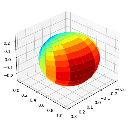
[4]:
(<Figure size 960x480 with 1 Axes>, <Axes3D: >)
Generate Receiver Arrays
[5]:
# Antenna Array at UE side
# antenna element type to be "OMNI"
# with single panel and 4 single polarized antenna element per panel.
ueAntArray = AntennaArrays(antennaType = "OMNI",
                           centerFrequency = carrierFrequency,
                           arrayStructure  = np.array([1,1,2,2,1]))

ueAntArray()

# num of Rx antenna elements
nr = ueAntArray.numAntennas
# Radiation Pattern of Rx antenna element
ueAntArray.displayAntennaRadiationPattern()
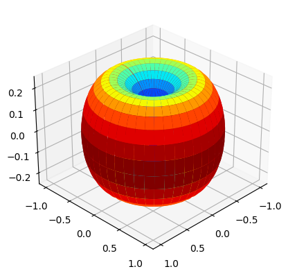
[5]:
(<Figure size 960x480 with 1 Axes>, <Axes3D: >)
Generate the Routes
Generate the BS Routes
[6]:
# NodeMobility parameters
# assuming that all the BSs are static and all the UEs are mobile.
# time values at each snapshot.
snapshotInterval = 10**-3/14 # 5 second
speed = 0.833 # speed of the UE 3 Kmph
radius = 250 # 3 Kmph
timeInst = snapshotInterval*np.arange(nSnapShots, dtype=np.float32)
typeOfMobility = "vehicle"
numVehicles = nBSs
timeInstances = timeInst
option = "optionA"
laneWidth = 10
numLanes = 2
vehicledropType = "random"
randomizeOrientations = False
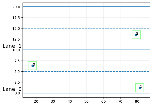
BSroute = NodeMobility(typeOfMobility, numVehicles, timeInstances, option,
laneWidth, numLanes, vehicledropType, randomizeOrientations)
BSroute()
BSroute.displayRoute()
# ax.set_aspect(True)
Generate the UE Routes
[7]:
# NodeMobility parameters
# assuming that all the BSs are static and all the UEs are mobile.
# time values at each snapshot.
snapshotInterval = 10**-3/14 # 5 second
speed = 0.833 # speed of the UE 3 Kmph
radius = 250 # 3 Kmph
timeInst = snapshotInterval*np.arange(nSnapShots, dtype=np.float32)
typeOfMobility = "vehicle"
numVehicles = nUEs
timeInstances = timeInst
option = "optionA"
laneWidth = 10
numLanes = 2
vehicledropType = "random"
randomizeOrientations = False
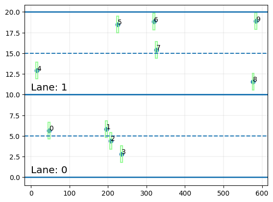
UEroute = NodeMobility(typeOfMobility, numVehicles, timeInstances, option,
laneWidth, numLanes, vehicledropType, randomizeOrientations)
UEroute()
UEroute.displayRoute()
# ax.set_aspect(True)
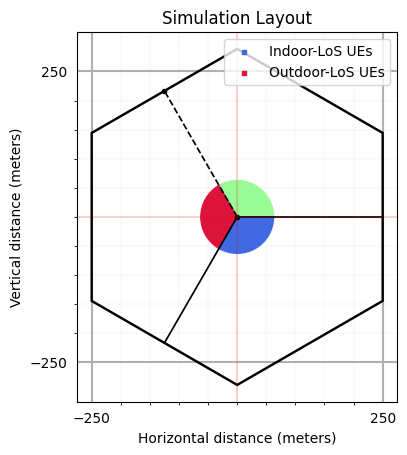
Simulation Layout
We define the simulation topology parametes:
ISD: Inter Site DistanceminDist: Minimum distance between transmitter and receiver.bsHt: BS heightsueHt: UE heightstopology: Simulation TopologynSectorsPerSite: Number of Sectors Per Site
Furthermore, users can access and update following parameters as per their requirements for channel using the handle simLayoutObj.x where x is:
The following parameters can be accessed or updated immendiately after object creation
UEtracksUELocationsueOrientationUEvelocityVectorBStracksBSLocationsbsOrientationBSvelocityVector
The following parameters can be accessed or updated after calling the object
linkStateVec
[8]:
# Layout Parameters
isd             = 500         # inter site distance
minDist         = 35          # min distance between each UE and BS
ueHt            = 1.5         # UE height
bsHt            = 35          # BS height
topology        = "Hexagonal" # BS layout type
nSectorsPerSite = 3           # number of sectors per site

memoryEfficient                = False
enableSpatialConsistencyLoS    = True
enableSpatialConsistencyIndoor = True


print("      enableSpatialConsistency: "+str(enableSpatialConsistencyLoS))
print("               memoryEfficient: "+str(memoryEfficient))
print("enableSpatialConsistencyIndoor: "+str(enableSpatialConsistencyIndoor))

# simulation layout object
simLayoutObj = SimulationLayout(numOfBS = nBSs,
                                numOfUE = nUEs,
                                heightOfBS = bsHt,
                                heightOfUE = ueHt,
                                ISD = isd,
                                layoutType = topology,
                                numOfSectorsPerSite = nSectorsPerSite,
                                ueRoute = UEroute,
                                bsRoute = BSroute,
                                memoryEfficient = memoryEfficient,
                                useInitueLocations= True,
                                enableSpatialConsistencyLoS = enableSpatialConsistencyLoS,
                                enableSpatialConsistencyIndoor = enableSpatialConsistencyIndoor)

# Update UE location for motion over a circle centered around the BS location.
simLayoutObj.UELocations = -simLayoutObj.UEtracks.mean(0)

simLayoutObj(terrain = propTerrain,
             carrierFreq = carrierFrequency,
             ueAntennaArray = ueAntArray,
             bsAntennaArray = bsAntArray,
             forceLOS = False)

# displaying the topology of simulation layout

fig, ax = simLayoutObj.display2DTopology()

ax.scatter(simLayoutObj.UELocations[0,0]+simLayoutObj.UEtracks[:,0,0],
           simLayoutObj.UELocations[0,1]+simLayoutObj.UEtracks[:,0,1],
           color="k", label = "NLoS Instants", zorder=-1)
ax.scatter(simLayoutObj.UELocations[0,0]+simLayoutObj.UEtracks[simLayoutObj.linkState[:,0,3],0,0],
           simLayoutObj.UELocations[0,1]+simLayoutObj.UEtracks[simLayoutObj.linkState[:,0,3],0,1],
           color="r", label = "LoS Instants", zorder=-1)
ax.scatter(simLayoutObj.UELocations[0,0],simLayoutObj.UELocations[0,1], color="b", label = "UE-InitialLocation", zorder=-3)
ax.set_xlabel("x-coordinates (m)")
ax.set_ylabel("y-coordinates (m)")
ax.set_title("Simulation Topology")
ax.legend()
# plt.show()
      enableSpatialConsistency: True
               memoryEfficient: False
enableSpatialConsistencyIndoor: True
[8]:
<matplotlib.legend.Legend at 0x7fb96d21c390>
Channel Parameters, Channel Coefficients and OFDM Channel
The user can access the channel coefficents and other parameters using following handles:
LSPs/SSPs: paramGenObj.x where x is
linkStateVecdelaySpreadphiAoA_LoS,phiAoA_mn,phiAoA_spreadthetaAoA_LoS,thetaAoA_mn,thetaAoA_spreadphiAoD_LoS,phiAoD_mn,phiAoD_spreadthetaAoD_LoS,thetaAoD_mn,thetaAoD_spreadxprpathloss,pathDelay,pathPowershadowFading
Channel Co-efficeints: channel.x where x is
coefficientsdelays
Shape of OFDM Channel:
Hfis of shape :(number of carrier frequencies, number of snapshots, number of BSs, number of UEs, Nfft, number of Rx antennas, number of Tx antennas)
[9]:
# Generate SSPs/LSPs Parameters:
paramGenObj = simLayoutObj.getParameterGenerator(memoryEfficient = True,
                                                 enableSpatialConsistencyForLSPs = True,
                                                 enableSpatialConsistencyForSSPs = True,
                                                 enableSpatialConsistencyForInitialPhases = True)

# Generate Channel Coefficeints and Delays: SSPs/LSPs
channel = paramGenObj.getChannel(applyPathLoss = True)
# Channel coefficients can be accessed using: channel.coefficients
# Channel delays can be accessed using:       channel.delays

# Generate OFDM Channel
Nfft = 1024
Hf   = channel.ofdm(30*10**3, Nfft, simLayoutObj.carrierFrequency)
[Warning]: Pathloss model for UMi is defined only for BS height 'hBS' = 10! Ignoring for now but might results in unexpected behaviour!
[Warning]: UE height 'hUE' cannot be less than 1.5! These values are forced to 1.5!
[Warning]: Pathloss model for UMi is defined only for  2D distances 'd2D' between 10m and 5Km! Some distances are from outside this interval!
Ignoring for now but might result in unexpected behaviour!
[10]:
Hf.shape
[10]:
(1, 14, 3, 10, 1024, 4, 4)
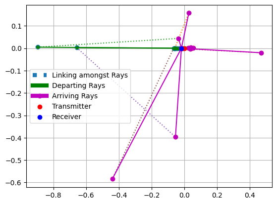
[11]:
fig, ax = paramGenObj.displayClusters(indices=(0, 1, 0), rayIndex=1, carrierIndex=0,
                                      radiusRx=10, radiusTx=10, displayPlot=False)
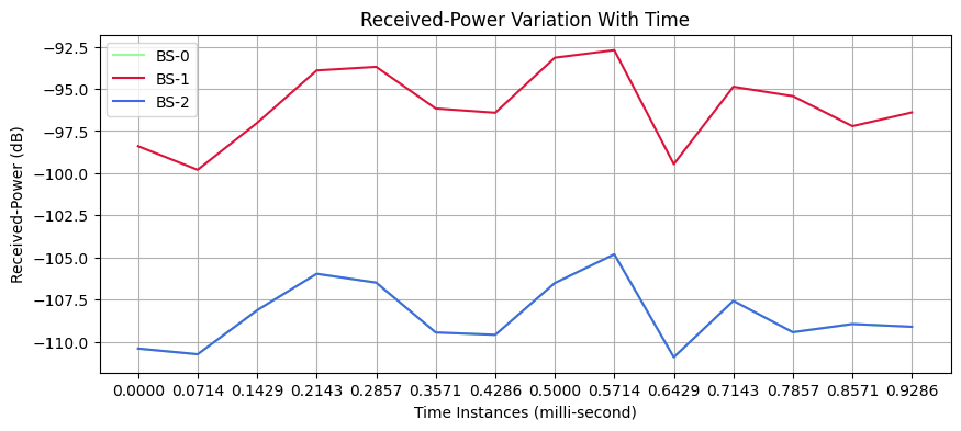
Variation in Channel Power across Time
The following code snippets displays the variation of received power of a UE when moves on a circular track (centered around origin) starting from its
initial position.In the current simulation we have 3 BSs and 1 UE moving on a circular track starting from a random intitial position inside a hexagonal layout.
[12]:
fig, ax = plt.subplots(figsize = (10,4))
power   = 10*np.log10(((np.abs(Hf)**2).sum(axis=0).sum(axis=2).sum(axis=2).sum(axis=2).sum(axis=2))/(nr*nt))
colors  = np.array(['palegreen', 'crimson','royalblue'])
ax.plot(timeInst*1000, power[:,0], colors[0], label = "BS-0")
ax.plot(timeInst*1000, power[:,1], colors[1], label = "BS-1")
ax.plot(timeInst*1000, power[:,2], colors[2], label = "BS-2")

ax.set_xticks(timeInst*1000)
ax.legend()
ax.grid()
ax.set_xlabel('Time Instances (milli-second)')
ax.set_ylabel('Received-Power (dB)')
ax.set_title('Received-Power Variation With Time', fontsize=12)

plt.show()
[ ]: