
Downlink TDoA Based Positioning for Industrial IoT Devices in Millimeter Wave 5G Networks
This tutorial estimates the position of based time of arrival estimates. The details of the tutorial simulation parameters is shown below:
Parameters |
Values |
|---|---|
Positioning Method |
DL-TDoA based |
Parameter Estimation Method |
ESPRIT |
Optimization Method |
Gradient Descent |
Carrier Frequency |
28 GHz |
Bandwidth |
150 MHz |
Subcarrier Spacing |
120 kHz |
Terrain |
Indoor-Factory (InF-SH) |
Channel State Information |
Zero Forcing + Spline Interpolation |
Reference Signal |
Positioning Reference Signal (PRS) |
Simulation Type |
System Level Simulation |
The tutorial will generate 5G standards compliant reference signal (PRS) which is transmitted by BS foe UE to perform measurement which inturn can be used to estimate the location of the UE. Users can generate the Wireless channel either using our tool which has one of the most exhaustive channel modelling library or use some other \(3^{rd}\) party tool such as Sionna, Quadriga to generate the channel and use it with 5G Toolkit.
Positioning Procedure
Generate the Reference Signal
Transmit the Reference Signal
Pass the Transmit Signal through Wireless Channel
Add Noise at the Receiver
Estimate the Channel at Pilot Locations
Interpolate the channel at remaining locations
Estimate the Delays (Time of arrival using the channel Estimates)
Estimate the Position using ToA estimates.
Select the most accurate measurements for Positioning.
Compute Time Difference of Arrival (TDoA) measurements.
Estimate position of the UEs based on TDoA measurements.
Finally, we will demonstrate the efficacy of these methods using simulation evaluation results:
Horizontal (2D) Positioning Accuracy vs SNR
Verical Positioning Accuracy vs SNR
3D Positioning Accuracy
Table of Content:
Position Estimation + K-Best Measurement Selection (Genie Aided)
Performance Analysis of Positioning Error for ToA based method
Import Libraries
Python Libraries
[1]:
# from IPython.display import display, HTML
# display(HTML("<style>.container { width:100% !important; }</style>"))
import os
os.environ["CUDA_VISIBLE_DEVICES"] = "-1"
os.environ['TF_CPP_MIN_LOG_LEVEL'] = '3'
# %matplotlib widget
import matplotlib.pyplot as plt
import matplotlib.patches as mpatches
import matplotlib as mpl
import numpy as np
from scipy import interpolate
5G Toolkit Libraries
[2]:
import sys
sys.path.append("../../../")
from toolkit5G.ChannelModels import AntennaArrays, SimulationLayout, ParameterGenerator, ChannelGenerator
from toolkit5G.ResourceMapping import ResourceMapperPRS
from toolkit5G.Positioning import ToAEstimation, LeastSquareTDoA, LeastSquareToA
from toolkit5G.ChannelProcessing import AddNoise
Simulation Parameters
Parameters |
Values |
|---|---|
Terrain |
Indoor Factory Sparse High (InF-SH) |
Carrier Frequency |
28 GHz |
Subcarrier Spacing |
30 kHz |
Number of Base-station |
21 (7 sites with 3 sectors each) |
BS Deployment |
Hexagonal |
UE Dropping |
Uniformly at random in the hall |
Number of UEs |
100 |
Bandwidth |
30 MHz (85 RBs) |
Number of RBs |
85 |
[3]:
propTerrain = "InF-SH" # Propagation Scenario or Terrain for BS-UE links
carrierFrequency = 28*10**9 # Array of two carrier frequencies in GHz
scs = 120*10**3
Nfft = 1024
numOfBSs = np.array([6,3], dtype=int) # number of BSs
nBSs = 18 # np.prod(numOfBSs)
nUEs = 100 # number of UEs
Bandwidth = 150*(10**6)
numRBs = 85
print()
print("*****************************************************")
print(" Terrain: "+str(propTerrain))
print(" Number of UEs: "+str(nUEs))
print(" Number of BSs: "+str(numOfBSs))
print(" carrier Frequency: "+str(carrierFrequency/10**9)+" GHz")
print(" Bandwidth: "+str(Bandwidth))
print(" Number of Resource Blocks: "+str(numRBs))
print(" Subcarrier Spacing: "+str(scs))
print(" FFT Size: "+str(Nfft))
print("*****************************************************")
print()
*****************************************************
Terrain: InF-SH
Number of UEs: 100
Number of BSs: [6 3]
carrier Frequency: 28.0 GHz
Bandwidth: 150000000
Number of Resource Blocks: 85
Subcarrier Spacing: 120000
FFT Size: 1024
*****************************************************
Channel Generation
Channel Parameters:
Intersite Distance: 200m
BS is deployed at 35m and UE has a random height between 0 and 1.5m.
BS Antennas Arrays:
Antenna Types: Parabolic
Number of Panels: 1
Number of Antennas: 2 Horizontally, 2 Verically
Polarization: 1 (Monopole)
UE Antennas Arrays:
Antenna Types: Hertizian (Omni)
Number of Panels: 1
Number of Antennas: 4 Horizontally, 4 Verically
Polarization: 1 (Monopole)
Mobility: No Mobility
OFDM Channel:
Carrier Phase: Disabled.
\(\text{N}_\text{fft}\): 1024
[4]:
# Antenna Array at UE side
# assuming antenna element type to be "OMNI"
# with 2 panel and 2 single polarized antenna element per panel.
ueAntArray = AntennaArrays(antennaType = "OMNI", centerFrequency = carrierFrequency,
arrayStructure = np.array([1,1,4,4,1]))
ueAntArray()
# # Radiation Pattern of Rx antenna element
# ueAntArray.displayAntennaRadiationPattern()
# Antenna Array at BS side
# assuming antenna element type to be "3GPP_38.901", a parabolic antenna
# with 4 panel and 4 single polarized antenna element per panel.
bsAntArray = AntennaArrays(antennaType = "3GPP_38.901", centerFrequency = carrierFrequency,
arrayStructure = np.array([1,1,2,2,1]))
bsAntArray()
# # Radiation Pattern of Tx antenna element
# bsAntArray[0].displayAntennaRadiationPattern()
# Layout Parameters
isd = 20 # inter site distance
minDist = 0 # min distance between each UE and BS
ueHt = 1.5 # UE height
bsHt = 3 # BS height
bslayoutType = "Rectangular" # BS layout type
ueDropType = "Rectangular" # UE drop type
htDist = "random" # UE height distribution
ueDist = "random" # UE Distribution per site
nSectorsPerSite = 1 # number of sectors per site
maxNumFloors = 3 # Max number of floors in an indoor object
minNumFloors = 1 # Min number of floors in an indoor object
heightOfRoom = 5.1 # height of room or ceiling in meters
indoorUEfract = 0.5 # Fraction of UEs located indoor
lengthOfIndoorObject = 3 # length of indoor object typically having rectangular geometry
widthOfIndoorObject = 3 # width of indoor object
forceLOS = True # boolen flag if true forces every link to be in LOS state
# forceLOS = False # boolen flag if true forces every link to be in LOS state
# simulation layout object
simLayoutObj = SimulationLayout(numOfBS = numOfBSs,
numOfUE = nUEs,
heightOfBS = bsHt,
heightOfUE = ueHt,
ISD = isd,
layoutType = bslayoutType,
layoutWidth = 50,
layoutLength = 120,
ueDropMethod = ueDropType,
UEdistibution = ueDist,
UEheightDistribution = htDist,
numOfSectorsPerSite = nSectorsPerSite,
ueRoute = None)
simLayoutObj(terrain = propTerrain,
carrierFreq = carrierFrequency,
ueAntennaArray = ueAntArray,
bsAntennaArray = bsAntArray,
indoorUEfraction = indoorUEfract,
heightOfRoom = heightOfRoom,
lengthOfIndoorObject = lengthOfIndoorObject,
widthOfIndoorObject = widthOfIndoorObject,
maxNumberOfFloors = maxNumFloors,
forceLOS = forceLOS)
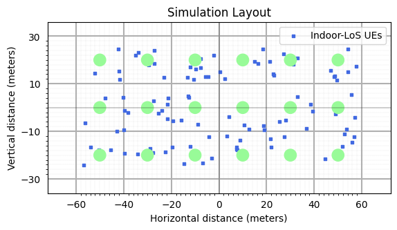
# displaying the topology of simulation layout
fig, ax = simLayoutObj.display2DTopology()
ax.set_xlabel("x-coordinates (m)")
ax.set_ylabel("y-coordinates (m)")
ax.set_title("Simulation Topology")
# ax.axhline(y=-0.5*isd*numOfBSs[1], xmin=10/140, xmax=130/140, color="k")
# ax.axhline(y= 0.5*isd*numOfBSs[1], xmin=10/140, xmax=130/140, color="k")
# ax.axvline(x=-0.5*isd*numOfBSs[0], ymin=10/140, ymax=130/140, color="k")
# ax.axvline(x= 0.5*isd*numOfBSs[0], ymin=10/140, ymax=130/140, color="k")
paramGen = simLayoutObj.getParameterGenerator(muKdB=-9, sigmaKdB=0.25)
# paramGen.displayClusters((0,0,0), rayIndex = 0)
channel = paramGen.getChannel()
Hf = channel.ofdm(scs, Nfft)[0]
Nt = bsAntArray.numAntennas # Number of BS Antennas
Nr = ueAntArray.numAntennas
[5]:
bsAntArray.displayAntennaRadiationPattern()
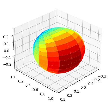
[5]:
(<Figure size 960x480 with 1 Axes>, <Axes3D: >)
Position Reference Signal
Number of OFDM symbols occupied by PRS:
dl_PRS_NumSymbolsCOMB size-N for PRS Transmission:
dl_PRS_CombSizeNPRS symbol offset:
dl_PRS_ResourceSymbolOffsetResource Element offset in PRS:
dl_PRS_ReOffsetPRS Resource-ID:
dl_PRS_SequenceIDIndex of the Slot which will carry the PRS resource Grid:
slotNumberPower scaling factor of PRS per ofdm symbol:
betaPRSPRS Resource Grid: (prsGrid) - \(\text{N}_\text{BS} \times 14*\text{numSlots} \times 12*\text{numRBs}\)
[6]:
dl_PRS_NumSymbols = 12 # Number of OFDM symbols occupied by PRS
dl_PRS_CombSizeN = 12 #12 # COMB size-N
dl_PRS_ResourceSymbolOffset = 0 # PRS symbol offset
dl_PRS_ReOffset = 0 # RE offset in PRS # not considered
dl_PRS_SequenceID = 231 # PRS Sequence ID.
# Number of slots per frame
numBSsPerSlot = dl_PRS_CombSizeN
numSlots = int(np.ceil(nBSs/numBSsPerSlot))
slotNumber = 15 # Index of slot where the PRS is loaded
betaPRS = 0.5 # power scaling factor of PRS per ofdm symbol
prsGrid = np.zeros((nBSs, numSlots, 14, numRBs*12), dtype = np.complex64)
prsObject = np.empty((nBSs), dtype=object)
resGrid = np.zeros((numSlots, 14, 12), dtype = np.int8)
for nbs in range(nBSs):
# Object for generating the PRS Resource Grid
slotIndex = int(nbs/numBSsPerSlot)
prsObject[nbs] = ResourceMapperPRS(betaPRS, dl_PRS_CombSizeN, dl_PRS_ReOffset + int(nbs%numBSsPerSlot),
dl_PRS_ResourceSymbolOffset, dl_PRS_NumSymbols, dl_PRS_SequenceID+nbs)
# Generate the PRS Resource Grid
prsGrid[nbs, slotIndex] = prsObject[nbs](slotNumber+slotIndex, numRBs)
resGrid[slotIndex] = resGrid[slotIndex] + np.round(np.abs(prsGrid[nbs, slotIndex]))[:,0:12]*(nbs+1)
prsGrid = prsGrid.reshape(nBSs, -1, numRBs*12)
resGrid = resGrid.reshape(-1, 12)
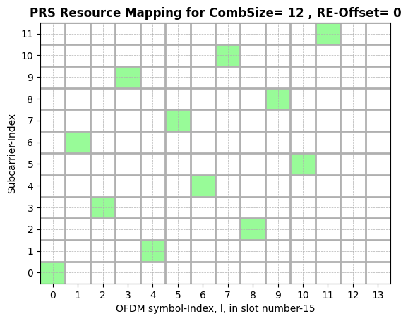
[7]:
f,a = prsObject[0].displayResourceGrid() # Display PRS Resource Grid
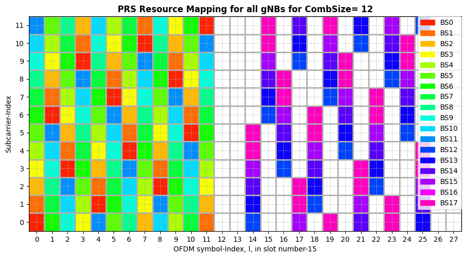
[8]:
fig, ax = plt.subplots(figsize=(11,5.5))
colors = ['white', 'red', 'lightcoral', 'gold', 'midnightblue', 'purple','black','darkorange', 'green', 'magenta', 'brown', 'yellow', 'pink']
bounds = np.arange(1, nBSs+1)
bounds = np.append([0], bounds)
cmap = plt.get_cmap('gist_rainbow')
colors = cmap(np.linspace(0,1,nBSs+1))
colors[0] = 0
option = "limited"
combSize = dl_PRS_CombSizeN
cmap = mpl.colors.ListedColormap(colors)
norm = mpl.colors.BoundaryNorm(bounds, cmap.N)
ax.imshow(np.abs(resGrid.T), interpolation='none', cmap=cmap, norm=norm, aspect = "auto", origin='lower')
ax.set_yticks(np.arange(0.5, 12, 1), minor=True);
ax.set_yticks(np.arange(0, 12, 1), minor=False);
ax.set_xticks(np.arange(0.5, 14*numSlots, 1), minor=True);
ax.set_xticks(np.arange(0, 14*numSlots, 1), minor=False);
ax.tick_params(axis='both',which='minor', grid_linewidth=2, width=0)
ax.tick_params(axis='both',which='major', grid_linewidth=0.5, grid_linestyle = '--')
ax.set_title("PRS Resource Mapping for all gNBs for CombSize= "+str(combSize), fontweight ='bold')
ax.set_xlabel('OFDM symbol-Index, l, in slot number-'+str(slotNumber))
ax.set_ylabel('Subcarrier-Index')
patches = [ mpatches.Patch(color=colors[i], label="BS"+str(i-1)) for i in range(1,nBSs+1) ]
# put those patched as legend-handles into the legend
ax.legend(handles=patches, loc='best', borderaxespad=0. )
plt.grid(which='both')
plt.show()
OFDM Transmitter: Create Transmission Grid
Transmission Grid:
XGridBandwidth RE Offset:
bwpOffset
[9]:
XGrid = np.zeros((nBSs, 14*numSlots, Nfft), dtype = np.complex64)
bwpOffset = np.random.randint(Nfft-numRBs*12)
## Load the resource grid to Transmission Grid
XGrid[...,bwpOffset:(bwpOffset+numRBs*12)] = prsGrid
print()
print("*****************************************************")
print(" Size of the Transmission Grid: "+str(XGrid.shape))
print(" BWP Resoure Element Offset: "+str(bwpOffset))
print(" Size of the PRS-Resource Grid: "+str(prsGrid.shape))
print("*****************************************************")
print()
*****************************************************
Size of the Transmission Grid: (18, 28, 1024)
BWP Resoure Element Offset: 0
Size of the PRS-Resource Grid: (18, 28, 1020)
*****************************************************
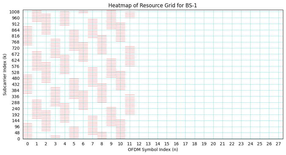
Display Transmission Grid
[10]:
# Plot Resource Grid
#################################################################
bsIndex = 1
fig, ax = plt.subplots(figsize=(11,5.5))
colors = ['palegreen', 'white', 'lightcoral', 'gold', 'midnightblue', 'purple']
bounds = [-1, 0, 1, 2, 3, 4, 5]
cmap = mpl.colors.ListedColormap(colors)
norm = mpl.colors.BoundaryNorm(bounds, cmap.N)
ax.imshow(np.round(np.abs(XGrid[bsIndex].T)), cmap = cmap, interpolation='none',
norm=norm, aspect = "auto", origin='lower')
ax.set_yticks(np.arange(0.5, 12*numRBs, 48), minor=False);
# ax.set_yticks(np.arange(0, 12, 1), minor=False);
# ax.set_xticks(np.arange(0.5, 14*numSlots, 1), minor=True);
ax.set_xticks(np.arange(0, 14*numSlots, 1), minor=False);
# ax.tick_params(axis='both',which='minor', grid_linewidth=2, width=0)
ax.tick_params(axis='both',which='major', grid_alpha = 0.75,
grid_linewidth=0.05, width=0, grid_linestyle = '--')
ax.set_xlabel("OFDM Symbol Index (n)")
ax.set_ylabel("Subcarrier Index (k)")
ax.set_title("Heatmap of Resource Grid for BS-"+str(bsIndex))
ax = plt.gca()
ax.grid(color='c', linestyle='--', linewidth=0.5)
# Gridlines based on minor ticks
plt.show()
Transmit Beamforming
Transmit Power, \(P_t\) (dBm)
Inter-Antenna spacing, d (m)
Beamformed Grid, Xf
Beamforming Direction: (0,0)
Note: Beam sweeping using multiple PRS significantly improves the positioning accuracy.
[11]:
#################################################################
# Bemforming angles
# Inter-element spacing in vertical and horizontal
Pt_dBm= 43
Pt = 10**(0.1*(Pt_dBm-30))
lamda = 3*10**8/carrierFrequency
d = 0.5/lamda
theta = 0
# Wt = np.sqrt(Pt/Nt)*np.exp(1j*2*np.pi*d*np.cos(theta)/(lamda*Nt)*np.arange(0,Nt))
# Xf = Wt.reshape(-1,1,1)*XGrid1
Xf = np.sqrt(dl_PRS_CombSizeN*Pt/Nt)*XGrid[..., np.newaxis].repeat(Nt, axis = -1)
print(" Beamformed Grid: "+str(Xf.shape))
Beamformed Grid: (18, 28, 1024, 4)
[12]:
Hf.shape
[12]:
(1, 18, 100, 1024, 16, 4)
Pass the Beamformed Grid Through Wireless Channel
OFDM Channel, Hf: (Number of Symbols (1), Number of BSs, Number of UEs, Nfft, Number of Rx Antennas, Number Tx Antennas)
Transmit Grid, Xf: (Number of BSs, Number of Tx Antennas, Number of Symbols, Nfft)
Received Grid, Y: (Number of UEs, Number of Rx Antennas, Number of Symbols, Nfft)
Note: Static Wireless Channel (No mobility is considered)
[13]:
Y = np.zeros((nUEs, Nr, 14*numSlots, Nfft), dtype=np.complex64)
for lbs in range(nBSs):
for lue in range(nUEs):
Y[lue] = Y[lue] + (Hf[0,lbs, lue][:,np.newaxis,...]@Xf[lbs].transpose(1,0,2)[...,np.newaxis])[...,0].transpose(-1,1,0)
print()
print("*****************************************************")
print(" Size of the Channel: "+str(Hf.shape))
print("Size of the Transmited Signal: "+str(Xf.shape))
print(" Size of the Received Signal: "+str(Y.shape))
print("*****************************************************")
print()
*****************************************************
Size of the Channel: (1, 18, 100, 1024, 16, 4)
Size of the Transmited Signal: (18, 28, 1024, 4)
Size of the Received Signal: (100, 16, 28, 1024)
*****************************************************
Add Noise
Noise Variance: \(k_B\) * T * B where
\(k_B\): Boltzmann Constant: \(1.380649 \times 10^{-23}\)
T: Temperature: 300 K
B: Bandwidth: 30 MHz
Carrier Frequency Offset: Not considered in this simulation
kppm (CFO in ppm of carrier frequency): 0
CFO
Received Grid with Noise (Yf)
[14]:
BoltzmanConst = 1.380649*(10**(-23))
temperature = 300
# noisePower = BoltzmanConst*temperature*Bandwidth
noisePower = BoltzmanConst*temperature*scs
kppm = 0
fCFO = kppm*(np.random.rand()-0.5)*carrierFrequency*(10**(-6)); # fCFO = CFO*subcarrierSpacing
CFO = (fCFO/scs)/Nfft
##Yf = AddNoise(True)(Y, noisePower, CFO)
Yf = AddNoise(False)(Y, noisePower, 0) #Added
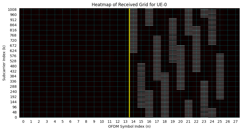
Extracting the Resource Grid
[15]:
rxGrid = Yf[...,bwpOffset:(bwpOffset+numRBs*12)]
[17]:
bsIndex = 0
ueIndex = 0
antIdx = 0
# Plot Resource Grid
#################################################################
fig, ax = plt.subplots(figsize=(11,5.5))
# colors = ['palegreen', 'white', 'lightcoral', 'gold', 'midnightblue', 'purple']
# bounds = [-1, 0, 1, 2, 3, 4, 5]
cmap = mpl.colors.ListedColormap(colors)
norm = mpl.colors.BoundaryNorm(bounds, cmap.N)
plt.imshow(np.abs(rxGrid[0,0].T), cmap = "hot", interpolation='none', aspect = "auto", origin='lower')
ax.axvline(x=13.5, color = 'y', lw = 3)
ax.set_yticks(np.arange(0.5, 12*numRBs, 48), minor=False);
# ax.set_yticks(np.arange(0, 12, 1), minor=False);
# ax.set_xticks(np.arange(0.5, 14*numSlots, 1), minor=True);
ax.set_xticks(np.arange(0, 14*numSlots, 1), minor=False);
# ax.tick_params(axis='both',which='minor', grid_linewidth=2, width=0)
ax.tick_params(axis='both',which='major', grid_alpha = 0.75,
grid_linewidth=0.05, width=0, grid_linestyle = '--')
ax.set_xlabel("OFDM Symbol Index (n)")
ax.set_ylabel("Subcarrier Index (k)")
ax.set_title("Heatmap of Received Grid for UE-"+str(ueIndex))
ax = plt.gca()
ax.grid(color='c', linestyle='--', linewidth=0.5)
# Gridlines based on minor ticks
plt.show()
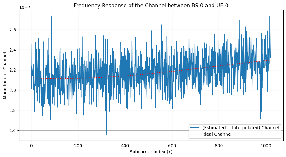
Channel Estimation + Interpolation
Channel estimation using zero-forcing/Least squares
Interpolation using spline interpolation from SciPy (splrep, splev)
Measurements across time are aggregated to improve the quality of channel estimates.
As the channel is no varying accross time.
[18]:
rxGrid = rxGrid.reshape(nUEs, Nr, numSlots, 14, numRBs*12)
prsGrid = prsGrid.reshape(nBSs, numSlots, 14, numRBs*12)
overSamplingFactor = 1
sA = 0
sP = 0
Hfest = np.zeros((nBSs, nUEs, Nr, 14, 12*numRBs), dtype=np.complex64)
Hfint = np.zeros((nBSs, nUEs, Nr, overSamplingFactor*12*numRBs), dtype=np.complex64)
for lbs in range(nBSs):
slotIndex = int(lbs/numBSsPerSlot)
for lue in range(nUEs):
# print("lbs, lue",lbs, lue)
for nr in range(Nr):
Hfest[lbs, lue, nr][prsObject[lbs].prsIndices] = rxGrid[lue, nr, slotIndex][prsObject[lbs].prsIndices]/prsGrid[lbs, slotIndex][prsObject[lbs].prsIndices]
H = np.sum(Hfest[lbs, lue, nr], axis = -2)
tck = interpolate.splrep(np.arange(0, overSamplingFactor*12*numRBs, overSamplingFactor), np.abs(H), s=sA)
amp = interpolate.splev( np.arange(0, overSamplingFactor*12*numRBs), tck, der=0)
tck = interpolate.splrep(np.arange(0, overSamplingFactor*12*numRBs, overSamplingFactor), np.unwrap(np.angle(H)), s=sP)
Hfint[lbs, lue, nr] = amp * np.exp(1j*interpolate.splev(np.arange(0, overSamplingFactor*12*numRBs), tck, der=0))
Display the quality of Channel Estimates
[19]:
bsIndex = 0
ueIndex = 0
antIdx = 0
fig, ax = plt.subplots(figsize=(11,5.5))
ax.plot(np.arange(bwpOffset, bwpOffset+12*numRBs, overSamplingFactor), np.abs(Hfint[bsIndex, ueIndex, antIdx]), label = "(Estimated + Interpolated) Channel")
ax.plot(np.arange(0, Nfft, 1), np.sqrt(dl_PRS_CombSizeN*Pt/Nt)*np.abs(np.sum(Hf[0,bsIndex, ueIndex][:,antIdx,:], axis= -1)), "r:", label = "Ideal Channel")
ax.legend(loc = 'best')
ax.set_xlabel("Subcarrier Index (k)")
ax.set_ylabel("Magnitude of Channel")
ax.set_title("Frequency Response of the Channel between BS-"+str(bsIndex)+" and UE-"+str(ueIndex))
ax.grid()
plt.show()
ToA Estimation
Parameters |
Values |
|---|---|
ToA Estimation Method |
ESPRIT |
Number of Path-delays estimated |
2 (incremented if ESPRIT doesn’t provide legit delays) |
Note:
ESPRIT has high time and memory-space complexity
But yeild better ToA estimates in comparison to MUSIC and DFT based based methods if sufficent diversity is avaiable across measurements (space diversity in this case).
Furthermore, it has very few hyper-parameters required to be passed as input.
[20]:
toaEstimation = ToAEstimation("ESPRIT", Hfint[0, 0].reshape(-1,overSamplingFactor*12*numRBs).T.shape)
ToAe = np.zeros(Hfint.shape[0:2])
Lpath = 3
for nbs in range(nBSs):
for nue in range(nUEs):
# print("(nbs, nue): ("+str(nbs)+", "+str(nue)+")")
delayEstimates = np.sort(toaEstimation(Hfint[nbs, nue].reshape(-1,overSamplingFactor*12*numRBs).T,
Lpath,
subCarrierSpacing = scs/overSamplingFactor))
delayEstimates = delayEstimates[delayEstimates > 0]
K = Lpath
while((delayEstimates.size==0) or (delayEstimates[0]<=0 and K < 12)):
K = K + 1
delayEstimates = np.sort(toaEstimation(Hfint[nbs, nue].reshape(-1,overSamplingFactor*12*numRBs).T,
numberOfPath = K,
subCarrierSpacing = scs/overSamplingFactor))
delayEstimates = delayEstimates[delayEstimates > 0]
if(delayEstimates.size == 0):
ToAe[nbs, nue] = 10**-9
else:
ToAe[nbs, nue] = delayEstimates[0]
Visualization: Time of Arrival locus Circles
Display the locus for all the circle with radius \(= 3 \times 10^{8} \times\) ToA. The circle denotes te possible location of UEs. The UE actually lies at the intersection of the circle drawn around the BS correspsonding to ToA-measurement for the specific UE.
[21]:
#################################################################
rxPosition = simLayoutObj.UELocations
txPosition = simLayoutObj.BSLocations
rangeEst_2D = np.sqrt(np.abs((ToAe*(3*10**8))**2 - (rxPosition[:,2].reshape(1,-1)-txPosition[:,2].reshape(-1,1))**2))
fig, ax = plt.subplots(figsize=(10,5))
ax.set_aspect(True)
colors = ["k","m","r","b","g","y","crimson"]
linestyle_tuple = ['solid', 'dotted', 'dashed', 'dashdot',
(0, (5, 10)), # 'loosely dashed'
(0, (1, 10)), # 'loosely dotted'
(5, (10, 3)), # 'long dash with offset'
(0, (5, 1)), # 'densely dashed'
(0, (3, 10, 1, 10)), # 'loosely dashdotted'
(0, (3, 5, 1, 5)), # 'dashdotted'
(0, (3, 1, 1, 1)), # 'densely dashdotted'
(0, (3, 5, 1, 5, 1, 5)), # 'dashdotdotted'
(0, (3, 10, 1, 10, 1, 10)), # 'loosely dashdotdotted'
(0, (3, 1, 1, 1, 1, 1))] # 'densely dashdotdotted'
for nbs in range(nBSs):
for nue in range(nUEs):
circle1 = plt.Circle((txPosition[nbs,0], txPosition[nbs,1]), rangeEst_2D[nbs,nue],
color = colors[nue%7], lw = 0.5, ls = linestyle_tuple[nue%7],
fill = False, zorder = 1)
ax.add_artist(circle1)
ax.scatter(txPosition[:,0], txPosition[:,1], marker="P", color="b", edgecolors='white', s = 200, label="Tx-Locations", zorder = 2)
ax.legend()
ax.set_xlabel("x-coordinates (m)")
ax.set_ylabel("y-coordinates (m)")
ax.set_title("Transmitter's Locations and ToA Locuses (Potential UE Locations)")
ax.grid(True)
plt.show()
#________________________________________________________________

Position Estimation + K-Best Measurement Selection (Genie Aided)
Measurement Selection:
Select the most accurate k ToA measnurements for Positioning
Even 1 Inaccuracte measurement can compromise the positioning performance.
Genie Aided Measurement Selection: Assumes that the accuracy of the each measurment is known somehow.
Selects the best ToA-measurements available to each UE from the BSs for estimating the location.
[22]:
# # Selection of k Most Accurate Measurements
# #################################################################
k = 4 # Select k-best measurements
error = (np.abs(ToAe-channel.delays[0,0,...,0])/channel.delays[0,0,...,0]) # Compute the ToA error in each measurement
bsIndices = (np.argsort(error,axis=0)[0:k]).T
positionEstimate = LeastSquareTDoA()
# positionEstimate = LeastSquareToA()
# Position Estimation Object:
# Positioning based on: TDoA
# Optimization Method: Least Square
rxPositionEstimate = np.zeros((nUEs,2,3))
rxStdEstimate = np.zeros((nUEs))
kBestIndices = np.zeros((nUEs, k), dtype = np.int8)
for nue in range(nUEs):
toa = ToAe[bsIndices[nue],nue]
tdoa = toa[1::] - toa[0]
rxPositionEstimate[nue], rxStdEstimate[nue] = positionEstimate(txPosition[bsIndices[nue]], tdoa=tdoa)
# rxPositionEstimate[nue], rxStdEstimate[nue] = positionEstimate(txPosition[bsIndices[nue]], toa)
# print("nue: "+str(nue)+" | Rx Location Estimate: "+str(rxPositionEstimate[nue,0]))
Visualization of Positioning
Show the accurcy of positioning by comparing the actual location against the true location.
Disclaimer: Works well only if the intractive matplotlib is enabled
[23]:
rangeEst_2D = np.sqrt(np.abs((ToAe*(3*10**8))**2 - (rxPosition[:,2].reshape(1,-1)-txPosition[:,2].reshape(-1,1))**2))
# fig, ax = plt.subplots()
fig, ax = simLayoutObj.display2DTopology(isEqualAspectRatio = True)
colors = ["k","m","r","b","g","y","crimson"]
linestyle_tuple = ['solid', 'dotted', 'dashed', 'dashdot',
(0, (5, 10)), # 'loosely dashed'
(0, (1, 10)), # 'loosely dotted'
(5, (10, 3)), # 'long dash with offset'
(0, (5, 1)), # 'densely dashed'
(0, (3, 10, 1, 10)), # 'loosely dashdotted'
(0, (3, 5, 1, 5)), # 'dashdotted'
(0, (3, 1, 1, 1)), # 'densely dashdotted'
(0, (3, 5, 1, 5, 1, 5)), # 'dashdotdotted'
(0, (3, 10, 1, 10, 1, 10)), # 'loosely dashdotdotted'
(0, (3, 1, 1, 1, 1, 1))] # 'densely dashdotdotted'
# for nbs in range(k):
# for nue in range(nUEs):
# circle1 = plt.Circle((txPosition[kBestIndices[nue, nbs], 0], txPosition[kBestIndices[nue, nbs], 1]), rangeEst_2D[kBestIndices[nue, nbs], nue],
# color = colors[nue%7], lw = 0.35, ls = linestyle_tuple[nue%7], fill = False, zorder = 0)
# ax.add_artist(circle1)
ax.scatter(txPosition[:,0], txPosition[:,1], marker="P", color="b", edgecolors='white',
s = 125, label="Tx-Locations", zorder = 3)
ax.scatter(rxPositionEstimate[:,0,0], rxPositionEstimate[:,0,1], marker="o", color="g",
s = 75, label="Estimated Rx-Locations", zorder = 1)
ax.scatter(rxPosition[:,0], rxPosition[:,1], marker=".", color="r", edgecolors='white',
s = 100, label="True Rx-Locations", zorder = 2)
ax.legend()
ax.set_xlabel("x-coordinates (m)")
ax.set_ylabel("y-coordinates (m)")
ax.set_title("Transmitter's Locations and Estimation Accuracy (True UE Location vs Estimated UE Locations)")
ax.set_xlim([-75, 75])
ax.set_ylim([-30, 30])
ax.grid(True)

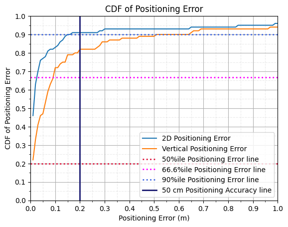
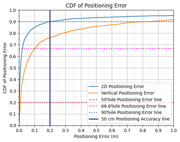
Performance Analysis of Positioning Error for ToA based method
The perfrormance of the positioning methods is analyzed using:
50 percentile Position Error in Horizontal and Vertical Direction.
67 percentile Position Error in Horizontal and Vertical Direction.
90 percentile Position Error in Horizontal and Vertical Direction.
Fraction of users which are positioned with accuracy better ththan 50 cm.
It can be easily observed that:
Error Percentile |
Horizontal Error |
Vertical Error |
|---|---|---|
50%ile |
8.5 cm |
13.5cm |
66%ile |
16.5cm |
20.0cm |
90%ile |
19.6cm |
33.1cm |
[24]:
nbins = nUEs
xlimit = 1
ylimit = 1
posError3D = np.linalg.norm(rxPositionEstimate[:, 0]-rxPosition, axis=1)
posError3D = np.where(np.isnan(posError3D), 0, posError3D)
posError2D = np.linalg.norm(rxPositionEstimate[:, 0, 0:2]-rxPosition[:, 0:2], axis=1)
# Horizontal Error
count, bins_count = np.histogram(posError2D, bins = nbins, range = [0, xlimit])
pdf = count/nUEs
cdf = np.cumsum(pdf)
fig, ax = plt.subplots()
ax.plot(bins_count[1:], cdf, label = "2D Positioning Error")
# Vertical Error
count, bins_count = np.histogram(posError3D, bins = nbins, range = [0, xlimit])
pdf = count/nUEs
cdf = np.cumsum(pdf)
ax.plot(bins_count[1:], cdf, label = "Vertical Positioning Error")
ax.set_xticks(np.linspace(0, xlimit, 11))
ax.set_xticks(np.linspace(0, xlimit, 21), minor=True)
ax.set_yticks(np.linspace(0, ylimit, 11))
ax.set_yticks(np.linspace(0, ylimit, 21), minor=True)
ax.set_xlabel("Positioning Error (m)")
ax.set_ylabel("CDF of Positioning Error")
ax.set_title("CDF of Positioning Error")
ax.axhline(y = 0.2, lw = 2, alpha = 1, linestyle = ':', color = "crimson", label = "50%ile Positioning Error line")
ax.axhline(y = 2/3, lw = 2, alpha = 1, linestyle = ':', color = "magenta", label = "66.6%ile Positioning Error line")
ax.axhline(y = 0.9, lw = 2, alpha = 1, linestyle = ':', color = "royalblue", label = "90%ile Positioning Error line")
ax.axvline(x = 0.2, lw = 2, alpha = 1, linestyle = '-', color = "midnightblue", label = "50 cm Positioning Accuracy line")
# Specify different settings for major and minor grids
ax.grid(which = 'minor', alpha = 0.25, linestyle = '--')
ax.grid(which = 'major', alpha = 1)
ax.set_xlim([0,xlimit])
ax.set_ylim([0,1])
ax.legend()
plt.show()
# # Code to save the Database
# idx = 0
# flag = True
# while(flag):
# print("flag: "+str(idx)+" | i="+str(idx))
# filename = "Databases/DLTDoA-"+str([idx])+".npz"
# if(os.path.exists(filename)):
# idx = idx + 1
# else:
# np.savez(filename, posError3D = posError3D, posError2D = posError2D,
# rxPositionEstimate = rxPositionEstimate, rxPosition = rxPosition,
# ToAe = ToAe, txPosition = txPosition, propTerrain = propTerrain,
# carrierFrequency = carrierFrequency, scs = scs, Nfft = Nfft,
# nBSs = nBSs, nUEs = nUEs, numRBs = numRBs,
# bsArrayStructure = np.array([1,1,2,2,1]),
# ueArrayStructure = np.array([1,1,4,4,1]))
# flag = False
flag: 0 | i=0
flag: 1 | i=1
flag: 2 | i=2
flag: 3 | i=3
flag: 4 | i=4
Performance Analysis: For 2000 UEs
[25]:
filename = "Databases/DLTDoA-"+str([0])+".npz"
ds = np.load(filename)
posError3D = ds["posError3D"]
posError2D = ds["posError2D"]
for i in range(1,5):
filename = "Databases/DLTDoA-"+str([i])+".npz"
ds = np.load(filename)
posError3D = np.concatenate([posError3D, ds["posError3D"]])
posError2D = np.concatenate([posError2D, ds["posError2D"]])
nbins = posError2D.size
xlimit = 1
ylimit = 1
# Horizontal Error
count, bins_count = np.histogram(posError2D, bins = nbins, range = [0, xlimit])
pdf = count/nbins
cdf = np.cumsum(pdf)
fig, ax = plt.subplots()
ax.plot(bins_count[1:], cdf, label = "2D Positioning Error")
# Vertical Error
count, bins_count = np.histogram(posError3D, bins = nbins, range = [0, xlimit])
pdf = count/nbins
cdf = np.cumsum(pdf)
ax.plot(bins_count[1:], cdf, label = "Vertical Positioning Error")
ax.set_xticks(np.linspace(0, xlimit, 11))
ax.set_xticks(np.linspace(0, xlimit, 21), minor=True)
ax.set_yticks(np.linspace(0, ylimit, 11))
ax.set_yticks(np.linspace(0, ylimit, 21), minor=True)
ax.set_xlabel("Positioning Error (m)")
ax.set_ylabel("CDF of Positioning Error")
ax.set_title("CDF of Positioning Error")
ax.axhline(y = 0.2, lw = 2, alpha = 1, linestyle = ':', color = "crimson", label = "50%ile Positioning Error line")
ax.axhline(y = 2/3, lw = 2, alpha = 1, linestyle = ':', color = "magenta", label = "66.6%ile Positioning Error line")
ax.axhline(y = 0.9, lw = 2, alpha = 1, linestyle = ':', color = "royalblue", label = "90%ile Positioning Error line")
ax.axvline(x = 0.2,lw = 2, alpha = 1, linestyle = '-', color = "midnightblue", label = "50 cm Positioning Accuracy line")
# Specify different settings for major and minor grids
ax.grid(which = 'minor', alpha = 0.25, linestyle = '--')
ax.grid(which = 'major', alpha = 1)
ax.set_xlim([0,xlimit])
ax.set_ylim([0,ylimit])
ax.legend()
plt.show()
[ ]:
# fig.savefig("IOO_20m_FR1.svg", transparent=False, format = "svg")
# fig.savefig("IOO_20m_FR1.png", transparent=False, format = "png")
Further Study
The tutorial can be extended further to study the effect of:
Subcarrier Spacing (\(\Delta f\))
Carrier Frequency (\(f_c\))
Bandwidth (\(B\))
NLoS Probability (\(p_{LOS}\))
Transmitter Power (\(P_t\))
Number of Base-stations (\(N_{BS}\))
Comb-factor (\(K_{comb}\))
on positioning accuracy. Furthermore, different terrians have different propagation characteristics. These characteristics effect the accuracy of positioning.
Thanks for reading the tutorial!
[ ]: