Watch on YouTube

View on GitHub

Download notebook

Analyzing the Impact of Scheduling Strategy on Blocking Probability

• In this notebook, we simulate the impact of scheduling strategy on blocking probability

• Base Station (BS) scheduler allocates different set of CCEs to different UEs based on a certain strategy

• For instance, let us consider two scheduling strategies namely strategy 1 and strategy 2, where

  • strategy 1: scheduler allocates UEs from low-to-high ALs. i.e., UEs with lower AL are scheduled first.

  • strategy 2: scheduler allocates UEs from high-to-low ALs. i.e., UEs with higher AL are scheduled first.

Python Libraries

import os
os.environ["CUDA_VISIBLE_DEVICES"] = "-1"
os.environ['TF_CPP_MIN_LOG_LEVEL'] = '3'

# %matplotlib widget
import matplotlib.pyplot  as plt
import matplotlib.patches as mpatches
import matplotlib as mpl

import numpy      as np

5G-Toolkit Libraries

import sys
sys.path.append("../../")
from toolkit5G.Scheduler import PDCCHScheduler

Simulation Parameters

The following parameters are used for this simulation: - coresetID denotes the coreset ID. - slotNumber denotes the slot-number carrying the PDCCH. - searchSpaceType denotes the search space type. UE specific search space (USS) or Common search space (CSS). - nci denotes the variable corresponding to carrier aggregation. Current simulation does not assume carrier aggregation.

mu                = np.random.randint(4)    # numerlogy for sub-carrier spacing
coresetID         = 1                       # coreset ID
slotNumber        = 0
searchSpaceType   = "USS"                   # search space type. UE specific search space
nci               = 0                       # variable corresponding to carrier aggregation
numIterations     = 1000

PDCCH Scheduling Parameters

Following parameters are crucial for PDCCH scheduling performance: - Nccep denotes coreset size or number of CCEs available for scheduling UEs. - strategy denotes the scheduling strategy. - numCandidatesUnderEachAL denotes number of PDCCH candidates per aggregation level. - aggLevelProbDistribution denotes the probability distribution with which the scheduler chooses a particular aggregation level (AL) for each UE. Supported ALs under USS are 1,2,4,8,16.

Nccep                    = 54
maxNumUEs                = 40
numUEs                   = np.arange(5,maxNumUEs+1,5)
aggLevelProbDistribution = np.array([0.4, 0.3, 0.2, 0.05, 0.05])
numCandidates            = np.array([6,6,4,2,1], dtype=int)
pdcchSchedulerObj        = PDCCHScheduler(mu, slotNumber, coresetID, nci)

Simulation for Scheduling Strategy-I

##############
# Strategy 1
##############
strategy                   = "Conservative"
probOfBlockingForStrategy1 = np.zeros((numUEs.shape))

for n in range(numUEs.size):
    print("Simulating (n,numUEs) : "+str(n)+", "+str(numUEs[n]))
    prob      = 0
    for i in range(numIterations):
        ueALdistribution  = np.random.multinomial(numUEs[n], aggLevelProbDistribution)
        rnti              = np.random.choice( np.arange(1,65519+1), size = (numUEs[n],), replace=False)
        count             = pdcchSchedulerObj(Nccep,searchSpaceType,ueALdistribution,numCandidates,rnti,strategy)[0]
        numBlockedUEs     = np.sum(count)
        prob              = prob + numBlockedUEs/numUEs[n]
    probOfBlockingForStrategy1[n] = prob/numIterations

Simulating (n,numUEs) : 0, 5
Simulating (n,numUEs) : 1, 10
Simulating (n,numUEs) : 2, 15
Simulating (n,numUEs) : 3, 20
Simulating (n,numUEs) : 4, 25
Simulating (n,numUEs) : 5, 30
Simulating (n,numUEs) : 6, 35
Simulating (n,numUEs) : 7, 40

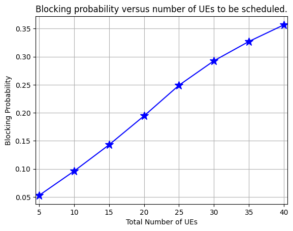
Blocking probability vs number of UEs to be scheduled.

• Its the recreation of Fig. 4: Blocking probability versus number of UEs to be scheduled. from the reference paper referenced below [1].

• Figure shows that by doubling the number of UEs from 15 to 30, the blocking probability increases from 0.15 to 0.3, corresponding to an increase by a factor of 2.

fig, ax = plt.subplots()
ax.plot(numUEs, probOfBlockingForStrategy1, marker  = "*",linestyle = "solid", ms = 12, c = 'b')

ax.set_xlabel('Total Number of UEs')
ax.set_ylabel('Blocking Probability')
ax.set_title('Blocking probability versus number of UEs to be scheduled.', fontsize=12)
ax.set_xticks(numUEs)
ax.set_xlim([numUEs[0]-0.5, numUEs[-1]+0.5])
ax.grid()
plt.show()

Simulation for Scheduling Strategy-II

##############
# Strategy 2
##############
strategy = "Aggressive"
probOfBlockingForStrategy2 = np.zeros((numUEs.shape))

for n in range(numUEs.size):
    print("Simulating (n,numUEs) : "+str(n)+", "+str(numUEs[n]))
    prob      = 0
    for i in range(numIterations):
        ueALdistribution  = np.random.multinomial(numUEs[n], aggLevelProbDistribution)
        rnti              = np.random.choice( np.arange(1,65519+1), size = (numUEs[n],), replace=False)
        count             = pdcchSchedulerObj(Nccep,searchSpaceType,ueALdistribution,numCandidates,rnti,strategy)[0]
        numBlockedUEs     = np.sum(count)
        prob              = prob + numBlockedUEs/numUEs[n]
    probOfBlockingForStrategy2[n] = prob/numIterations

Simulating (n,numUEs) : 0, 5
Simulating (n,numUEs) : 1, 10
Simulating (n,numUEs) : 2, 15
Simulating (n,numUEs) : 3, 20
Simulating (n,numUEs) : 4, 25
Simulating (n,numUEs) : 5, 30
Simulating (n,numUEs) : 6, 35
Simulating (n,numUEs) : 7, 40

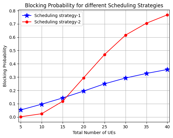
Plotting Blocking Probability vs Number of UEs for Scheduling Strategy

• Its the recreation of Fig. 10: Blocking probability for different scheduling strategiesfrom the paper referenced below [1].

• Figure shows that strategy 1 outperforms strategy 2 in terms of blocking probability.

• The reason is that strategy 2 prioritizes UEs with high ALs that uses more number of CCEs, thus resulting in a higher blocking probability compared to strategy 1.

• For instance, in strategy 2, a UE using AL 16 may block 16 UEs using AL 1.

• Also from the figure, we see that for a small number of UEs (e.g., 15) the two scheduling strategies have the same performance. However, when number of UEs increases to 40, blocking probability under strategy 2 is aproximately 3.5 times larger than the case with strategy 1, in the CORESET size of 54 CCEs.

• Note that the performance of different scheduling strategies is also dependent on the CORESET size.

fig, ax = plt.subplots()
ax.plot(numUEs, probOfBlockingForStrategy1, marker  = "*",linestyle = "solid", ms = 12, c = 'b', label = "Scheduling strategy-1")
ax.plot(numUEs, probOfBlockingForStrategy2, marker  = "o",linestyle = "solid", ms = 6,  c = 'r', label = "Scheduling strategy-2")

ax.legend()
ax.set_xlabel('Total Number of UEs')
ax.set_ylabel('Blocking Probability')
ax.set_title('Blocking Probability for different Scheduling Strategies', fontsize=12)
ax.set_xticks(numUEs)
ax.set_xlim([numUEs[0]-0.5, numUEs[-1]+0.5])
ax.grid()
plt.show()

References

[1] Blocking Probability Analysis for 5G New Radio (NR) Physical Downlink Control Channel. Mohammad Mozaffari, Y.-P. Eric Wang, and Kittipong Kittichokechai