
Wireless Channel Generation for Multiple Carrier Frequencies
In this tutorial, we will analyze the performance of channel Model at multiple carrier frequencies under the propagation scenario Urban Macro or “UMa” for a Hexagonal Base Station (BS) Layout.
For a given number of BSs and UEs we generate multi-frequency cluster level channel coefficients corresponding to every link being simulated.
We first import the necessary libraries then followed by creating objects of classes
AntennaArrays,NodeMobility, andSimulationLayoutrespectively.
The content of the tutorial is as follows:
Table of Contents
Import Libraries
Python Libraries
[1]:
import os
os.environ["CUDA_VISIBLE_DEVICES"] = "-1"
os.environ['TF_CPP_MIN_LOG_LEVEL'] = '3'

# %matplotlib widget
import matplotlib.pyplot as plt
import matplotlib as mpl
import numpy      as np
5G Toolkit Libraries
[2]:
# importing necessary modules for simulating channel model
# import sys
# sys.path.append("../../../")

from toolkit5G.ChannelModels import NodeMobility
from toolkit5G.ChannelModels import AntennaArrays
from toolkit5G.ChannelModels import SimulationLayout
from toolkit5G.ChannelModels import ParameterGenerator
from toolkit5G.ChannelModels import ChannelGenerator
Simulation Parameters
The simulation parameters are defined as follows * propTerrain defines propagation scenario or terrain for BS-UE, UE-UE, BS-BS links * carrierFrequency defines array of carrier frequencies in GHz * nBSs defines number of Base Stations (BSs) * nUEs defines number of User Equipments (UEs) * nSnapShots defines number of SnapShots
[3]:
# Simulation Parameters
propTerrain      = "UMa"                          # Propagation Scenario or Terrain for BS-UE links
carrierFrequency = np.array([3*10**9, 28*10**9])  # Array of two carrier frequencies in Hz
nBSs             = 21                             # number of BSs
nUEs             = 50                             # number of UEs
nSnapShots       = 10                             # number of SnapShots
Generate Antenna Array
Antenna Arrays for UEs
The following steps describe the procedure to simulate AntennaArrays Objects at a single carrier frequency both at Tx and Rx side:
[4]:
# Antenna Array at UE side
# assuming antenna element type to be "OMNI"
# with 2 panel and 2 single polarized antenna element per panel.
numCarriers = carrierFrequency.shape[0]
ueAntArray  = np.empty(numCarriers, dtype=object)
for i in range(carrierFrequency.size):
    ueAntArray[i] = AntennaArrays(antennaType     = "OMNI",
                                  centerFrequency = carrierFrequency[i],
                                  arrayStructure  = np.array([1,1,2,2,1]))
    ueAntArray[i]()
# Radiation Pattern of Rx antenna element
ueAntArray[0].displayAntennaRadiationPattern()
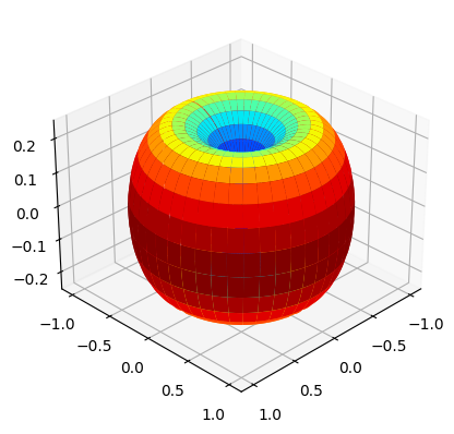
[4]:
(<Figure size 960x480 with 1 Axes>, <Axes3D: >)
[20]:
ueAntArray[0].displayArray("2D", markerSize = 288)
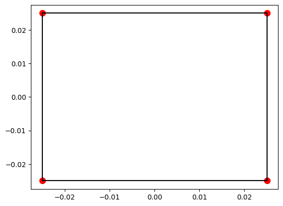
[20]:
(<Figure size 640x480 with 1 Axes>, <Axes: >)
Antenna Arrays for BS
[6]:
# Antenna Array at BS side
# assuming antenna element type to be "3GPP_38.901", a parabolic antenna
# with 4 panel and 4 single polarized antenna element per panel.
numCarriers    = carrierFrequency.shape[0]
bsAntArray     = np.empty(numCarriers, dtype=object)
for i in range(carrierFrequency.size):
    bsAntArray[i] = AntennaArrays(antennaType     = "3GPP_38.901",
                                  centerFrequency = carrierFrequency[i],
                                  arrayStructure  = np.array([1,1,4,4,1]))
    bsAntArray[i]()
# Radiation Pattern of Tx antenna element
bsAntArray[0].displayAntennaRadiationPattern()
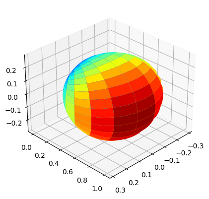
[6]:
(<Figure size 960x480 with 1 Axes>, <Axes3D: >)
[19]:
bsAntArray[0].displayArray("2D", markerSize = 288)
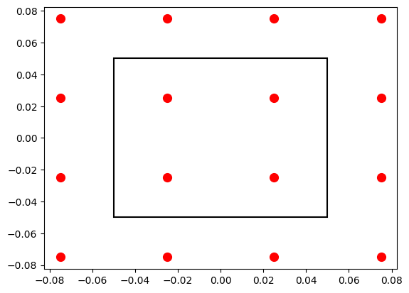
[19]:
(<Figure size 640x480 with 1 Axes>, <Axes: >)
Node Mobility
This subsection provides the following steps to simulate the mobility of each node
[8]:
# NodeMobility parameters
# assuming that all the BSs are static and all the UEs are mobile.
interval = 10*0.5*10**-3/nSnapShots
timeInst = np.arange(nSnapShots, dtype=np.float32)*interval  # time values at each snapshot.
UEroute  = NodeMobility("randomWalk", nUEs, timeInst, 0, 10)
UEroute.displayRoute()
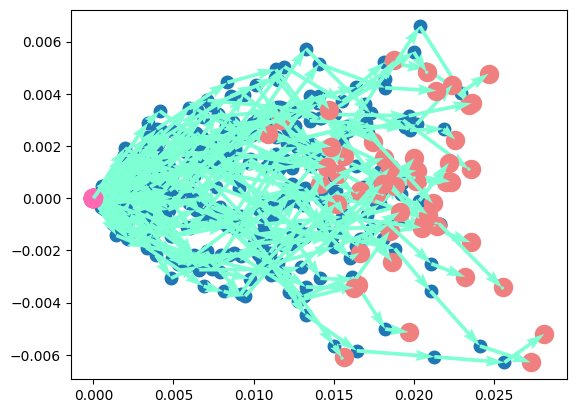
[8]:
(<Figure size 640x480 with 1 Axes>, <Axes: >)
Generate Simulation Layout
We define the simulation topology parametes:
ISD: Inter Site DistanceminDist: Minimum distance between transmitter and receiver.bsHt: BS heightsueHt: UE heightstopology: Simulation TopologynSectorsPerSite: Number of Sectors Per Site
Furthermore, users can access and update following parameters as per their requirements for channel using the handle simLayoutObj.x where x is:
The following parameters can be accessed or updated immendiately after object creation
UEtracksUELocationsueOrientationUEvelocityVectorBStracksBSLocationsbsOrientationBSvelocityVector
The following parameters can be accessed or updated after calling the object
linkStateVec
[9]:
# Layout Parameters
isd                  = 500         # inter site distance
minDist              = 35          # min distance between each UE and BS
ueHt                 = 1.5         # UE height
bsHt                 = 25          # BS height
bslayoutType         = "Hexagonal" # BS layout type
ueDropType           = "Hexagonal" # UE drop type
nSectorsPerSite      = 3           # number of sectors per site

# simulation layout object
simLayoutObj = SimulationLayout(numOfBS = nBSs,
                                numOfUE = nUEs,
                                heightOfBS = bsHt,
                                heightOfUE = ueHt,
                                UEheightDistribution="equal",
                                UEdistibution="equal",
                                ISD = isd,
                                layoutType = bslayoutType,
                                ueDropMethod = ueDropType,
                                numOfSectorsPerSite = nSectorsPerSite,
                                ueRoute = UEroute)

simLayoutObj(terrain = propTerrain,
             carrierFreq = carrierFrequency,
             ueAntennaArray = ueAntArray,
             bsAntennaArray = bsAntArray)

# displaying the topology of simulation layout
fig, ax = simLayoutObj.display2DTopology()
ax.set_xlabel("x-coordinates (m)")
ax.set_ylabel("y-coordinates (m)")
ax.set_title("Simulation Topology")
ax.legend()
[9]:
<matplotlib.legend.Legend at 0x7f4c0d32b050>
Generate Channel Parameters
This subsection provides the steps to obtain all the cluster level channel parameters, which includes both
Large Scale Parameters (LSPs)andSmall Scale Parameters (SSPs).LSPs includes
Path Loss (PL),Delay Spread (DS)andAngular Spreadsboth in Azimuth and Zenith directions, andcluster powers (Pn)comes under SSPs.LSPs/SSPs: paramGenObj.x where x is
linkStateVecdelaySpreadphiAoA_LoS,phiAoA_mn,phiAoA_spreadthetaAoA_LoS,thetaAoA_mn,thetaAoA_spreadphiAoD_LoS,phiAoD_mn,phiAoD_spreadthetaAoD_LoS,thetaAoD_mn,thetaAoD_spreadxprpathloss,pathDelay,pathPowershadowFading
[10]:
# channel parameters
paramGenObj = simLayoutObj.getParameterGenerator()
Generate Channel Coefficients
Cluster level channel coefficients can be simulated using the following code snippet.
channel.coefficientswith shape:(number of carrier frequencies, number of snapshots, number of BSs, number of UEs, numCluster/numPaths, number of Rx antennas, number of Tx antennas)channel.delayswith shape:(number of carrier frequencies, number of snapshots, number of BSs, number of UEs, numCluster/numPaths)
[11]:
channel = paramGenObj.getChannel(applyPathLoss = True)
Generate OFDM Channel
Shape of OFDM Channel:
Hfis of shape :(number of carrier frequencies, number of snapshots, number of BSs, number of UEs, fftsize, number of Rx antennas, number of Tx antennas)
[12]:
fftsize           = 512
subcarrierSpacing = 15*10**3
Hf = channel.ofdm(subcarrierSpacing, fftsize, simLayoutObj.carrierFrequency)
# Hf.shape: (numCarrierFrequencies, numSnapShots, numBSs, numUEs, Nfft, numRxAntennas, numTxAntennas)
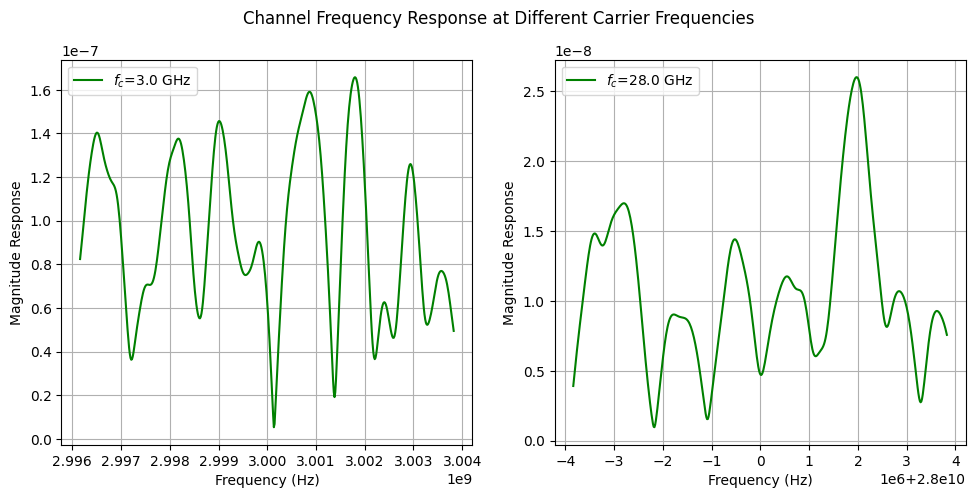
Frequency Domain : Magnitude Response Plot
The frequency domain magnitude plots (frequency responses) helps demonstate the order of frequency selectivity
Frequency selectivity is low for LOS Channel
frequency selectivity is high for NLOS Channels
Wireless channel at high frequency
has higher path-loss
less frequency selective (due to lower delay spread and weak distance paths)
[13]:
scaleFig = 1.5
fig, ax = plt.subplots(1,2,figsize=(17.5/scaleFig,7.5/scaleFig))
i = 0
ax[0].plot(np.arange(-channel.fftSize/2, channel.fftSize/2)*channel.subCarrierSpacing + channel.fc[0],
           np.abs(Hf[0,0,0,i,:,0,0]), "g", label = "$f_c$="+str(channel.fc[0]/10**9)+" GHz")

ax[1].plot(np.arange(-channel.fftSize/2, channel.fftSize/2)*channel.subCarrierSpacing + channel.fc[1],
           np.abs(Hf[1,0,0,i,:,0,0]), "g", label = "$f_c$="+str(channel.fc[1]/10**9)+" GHz")

ax[0].legend()
ax[0].set_xlabel("Frequency (Hz)")
ax[0].set_ylabel("Magnitude Response")
ax[0].grid()
ax[1].legend()
ax[1].set_xlabel("Frequency (Hz)")
ax[1].set_ylabel("Magnitude Response")
ax[1].grid()
fig.suptitle("Channel Frequency Response at Different Carrier Frequencies")

# plt.show()
[13]:
Text(0.5, 0.98, 'Channel Frequency Response at Different Carrier Frequencies')
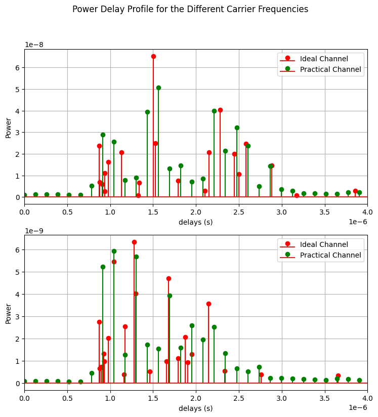
Time Domain Channel response
Practical wireless channel are bandlimited which results in:
impulses widening:
higher for lower frequency channels
time spread
These effects can be observed in following plots.
[14]:
ht = np.fft.ifft(Hf, fftsize, axis = -3)
[15]:
scaleFig = 2
fig, ax = plt.subplots(2,1,figsize=(17.5/scaleFig,17.5/scaleFig))
i = 0
ax[0].stem(channel.delays[0,0,0,i], np.abs(channel.coefficients[0,0,0,i,:,0,0]), "r", label = "Ideal Channel")
ax[0].stem(np.arange(fftsize)/(fftsize*channel.subCarrierSpacing), np.abs(ht[0,0,0,i,:,0,0]), "g", label = "Practical Channel")
ax[0].legend()
ax[0].set_xlim([0, 0.4*10**-5])
ax[0].set_xlabel("delays (s)")
ax[0].set_ylabel("Power")
ax[0].grid()

ax[1].stem(channel.delays[1,0,0,i], np.abs(channel.coefficients[1,0,0,i,:,0,0]), "r", label = "Ideal Channel")
ax[1].stem(np.arange(fftsize)/(fftsize*channel.subCarrierSpacing), np.abs(ht[1,0,0,i,:,0,0]), "g", label = "Practical Channel")
ax[1].legend()
ax[1].set_xlim([0, 0.4*10**-5])
ax[1].set_xlabel("delays (s)")
ax[1].set_ylabel("Power")
ax[1].grid()

fig.suptitle("Power Delay Profile for the Different Carrier Frequencies")
plt.show()
[ ]: